Analysis the Economic Efficiency of Common Beans Production among Smallholder Farmers: In Case of Burji District, Southern Nation National Peoples Region, Ethiopia
Tel: 910369238, Email: chanyalewmalle@gmail.com
Abstract
Production and productivity can be boosted either through increased use of inputs or by improving the efficiency of producers. The opportunities to increase farm production by bringing additional physical resource into cultivation have been diminishing. Then, reducing the existing inefficiency among farmers can be more effective. The serious reliance on obsolete farming techniques, poor complementary services such as extension, credit, marketing, infrastructure and poor and biased agricultural policies are among the major factors that have greatly constrained the development of Ethiopia's agriculture. This study tried to analyze the technical, allocative and economic efficiencies of common bean producer farmers in Burji district. It also identified the factors affecting the efficiency of producers in the study area. A multi-stage sampling technique was used to select 313 sample household farmers who were interviewed using a structured questionnaire to obtain data pertaining to common bean production during 2020. In the analysis, frontier 4.1 software was used to determine the levels of technical and economic efficiencies. Thus, the mean technical, allocative and economic efficiencies were 63.7, 77.2 and 50.0 percent respectively. Furthermore, descriptive statistics, stochastic frontier and two-limit Tobit regression models were employed. It was established from a stochastic frontier model that common bean yield estimated using Cobb- Douglas production function was positively influenced by seed, labor, oxen, land size, chemical and fertilizer (DAP). Similarly, a Tobit model revealed economic efficiencies was affected positively and significantly by family size, education, land size, TLU, access to credit, extension contact, training and off/none income. While variables such as crop pest affected negatively. Education, TLU, sex, access to credit, training, and off/none farm income influenced allocative efficiency positively and crop pest affected negatively. Finally, technical efficiency was affected age, family size, education, land size, sex, TLU, extension contact, training and off/none farm income affected technical efficiency positively while, distance from nearest market and crop pest affected it negatively. Thus, the study recommended policies targeting development of markets, roads and education of smallholder common bean producers that would promote economic efficiency of common bean producers.
Keywords
Common bean • Efficiency • Cobb-Douglas • Stochastic frontier • Two-limit Tobit regression
Abbreviations
AE: Allocative Efficiency; BWARDO: Burji Woreda Agriculture and Rural Development Office; CE: Cost Efficiency; CRS: Constant Returns to Scale; DEA: Data Envelopment Analysis; EE: Economic Efficiency; EIA: Ethiopian Institute of Agricultural Research; FAO: Food and Agricultural Organization; FAOSTAT: Food and Agricultural Organization Statistics; LR: Likelihood Ratio; MDE: Man Day Equivalent; MLE: Maximum Likelihood Estimator; MoA Minister of Agriculture; NGOs: Non-Governmental Organization; OLS: Ordinary Least Square; SFCF: Stochastic Frontier Cost Function; SFPF: Stochastic Frontier Production Function; SNNRS: Southern Nation National Regional State; TE: Technical Efficiency; TLU: Tropical Livestock Unit
Introduction
Legume seeds are an important staple foods and sources of dietary minerals that potentially provide all of the 15 essential minerals required by humans. Common bean (Phaseolus vulgaris L.) is the most vital grain legume for direct human consumption. The species has high diversity as seen in its morphological variability, uses and growth habits and patterns [1]. In the study area, common bean is known BURA BURJE and BOLOQE in the local Amharic language or Adenguare. It is a particularly important legume crop grown worldwide. It grows best in warm climates at temperatures of 18°C to 24°C [2].
This crop is currently estimated to be one of the most important legumes worldwide and it is described as a nearly "perfect" food. Nutritionally rich, it is also a good source of protein, dietary fiber and complex carbohydrates and it is an important source of nutrients for more than 300 million people in parts of Eastern Africa and Latin America, representing 65% of total protein consumed, 32% of energy and a major source of micronutrients, e.g., iron, zinc, thiamin and folic acid [3]. It is also important in nitrogen fixation thus improving the soil fertility as well as increasing crop production and improving the livelihoods of farmers [4]. It is described as a non-sensitive crop to soil as long as it is well-drained and fertile [5]. It can be growing successfully on most soil types, from light sands to heavy clays, but friable, deep and well-drained soils are best preferred [6].
According to Margaret et al., common bean in Sub-Saharan Africa (SSA) is an important crop for food-security and nutrition. It plays a big dietary role, supplying proteins, carbohydrates, essential elements and vitamins to both rural and urban households. It is estimated that the crop meets more than 50% of dietary protein requirements of households in SSA. The annual per capita consumption is higher among low-income people who cannot afford to buy nutritious food stuff, such as meats and fish [7].
Common bean is also a major food and cash crop in Ethiopia as well and it has considerable national economic significance. It is often grown as cash crop by small scale farmers and used as a major food legume in many parts of the country where it is consumed in different types of traditional dishes. It is cultivated in a wide range of agro-ecologies and farming systems including well-watered and drought-stressed areas [8].
This crop is distributed and grown in different parts of Ethiopia depending on climatic and socio-economic factors and is being part of the diets of the farming households; it serves as a source of protein to supplement the protein deficient main dishes like maize and Enset in the Southern parts of the country especially in Wolaita and Sidama areas. Besides, the farmers also grow common bean to use the straw as forage for livestock, source of fuel, mulching, bedding, and covering material for houses of poor farmers. In Ethiopia, the major common bean producing areas are Central, Eastern and Southern parts of the country [9].
Common bean (Phaseolus vulgaris L.) Production can increase either through introduction of modern technologies or by improving the efficiency of inputs with existing technologies. These two are not mutually exclusive, because the introduction of modern technology could not bring the expected shift of production frontier, if the existing level of efficiency is low. This implies that the need for the integration of modern technologies with improved level of efficiency. Therefore, a proper analysis of economic efficiency of farmers requires the estimation of both technical and allocative efficiencies.
In 2016/17 cropping season, in Ethiopia, common bean covered 290,202 hectares of land, and harvested 4,839,227 quintals of produce with productivity of 16.7 quintals per hectare and it was produced by around 4 million head house hold farmers in Ethiopia. When we come to the study area the production of common bean covered 2564 hectares of land, and harvested 26,922 quintals of produce with productivity of 10.5 quintals per hectare and it was produced by around 1463 head house hold farmers in 2019 production years [10].
Statement of the problem
The growing gap between common bean demand and supply in Ethiopia is mainly attributed to the very low productivity of the agricultural sector. The serious reliance on obsolete farming techniques, poor complementary services such as extension, credit, marketing, infrastructure and poor and biased agricultural policies are among the major factors that have greatly constrained the development of Ethiopia's agriculture. Farmers in the study area practice mixed farming system. Among the legumes grown in the study area, common bean is the major crop in terms of volume of the production and area cultivated. It is also the major source of cash income to the farmers among the crops grown in the area [11]. Accelerating the adoption of improved technologies by small-scale farmers is believed to result in higher output. However, the promoted technologies have not been used to full potential and no substantial gains could be achieved by using the technologies alone. Production inefficiency of smallholder farmers in Ethiopia has been one of the key factors limiting agricultural productivity especially that of pulse crops including common bean [12].
Therefore, in order to improve common bean production and productivity, it becomes vital to undertake economic efficiency analysis at farm level under the existing technology to enhance the contribution of the common bean sector to national economy. Moreover, identifying the extent of efficiency and the factors that contribute to it is of a paramount importance on the level of resource use efficiency in common bean production. Such information is useful for reducing the level of economic inefficiency.
Many people, in different sectors, have done efficiency studies in Ethiopia. However, much of these studies concentrated on the analysis of technical efficiency like [13]. Examination of the technical efficiency alone understates the benefits that could be derived by producers from improvements in overall performance. There are also few empirical studies in Ethiopia which have done economic efficiency analysis for different crops [14]. These major studies focused on major food crops like maize and wheat and also on vegetables. Hence, there is a need to fill the existing knowledge gap by addressing issues related to technical, allocative and economic efficiency of common bean production in Burji district providing empirical evidence from smallholder common bean producers. Therefore, the aim of this study gives better understanding on analysis of economic efficiency of common bean production in Burji special woreda, South nation national region Ethiopia by using extended efficiency measurement techniques.
Research questions
This study made an attempt to address the following main research questions:
• What is the level of technical, allocative and economic
efficiencies in common bean production of small-scale
common bean producers in Burji district?
• What are the sources/factors, which influence technical,
allocative and economic efficiency of small-scale common bean
producers in Burji district?
Objectives of the study
General objective: The general objective of this study was analyzing the economic efficiency of common bean in Burji district at Southern nation national region, Ethiopia.
Specific objectives: T he specific objectives of the study were:
• To measure the level of technical efficiency, allocative and
economic efficiency of common bean production in study area.
• To identify the factors affecting technical, allocative and eco nomic
efficiencies of common bean production in the study area.
Significance of the study
The measurement of efficiencies is a very important factor of productivity growth both in developing and developed countries. It is more so in developing agricultural economies where resources are meager and opportunities for developing and adopting better technologies have lately started dwindling [15]. The measurement of efficiency (TE, AE and EE) has a very significant importance for the Ethiopian economy as a whole. It is used to differentiate the inefficient farm and to derive lessons about better production practices from more efficient farms. Hence, this study believed to play a significant role in providing useful information regarding economic inefficiencies in production and helps to identify those factors, which are associated with inefficiencies that may exist. Besides, the study gives insight and serve as a document for students and researchers interested in the topic to stimulate further investigations of the problem in the study area.
The identification of the factors that determine the EE of common bean and determining the level of TE, AE and EE, has therefore, contribute to improve the farming practices of the studying area by giving relevant policy recommendations. Furthermore, given the fact that an efficiency study on common bean was not previously studied in Ethiopia, the results of this study will have a contribution to other developing countries.
Organization of the paper
This paper is organized into seven parts.
• Part one elaborate brief introduction of the study, statement of the
problem, research objectives, and research questions, scope of
the study and the importance of the study and paper organization.
• Part two gives theoretical and empirical.
• The third part gives the detailed methods and methodology in
which sample procedure and sample size determination be
pinpointed, how data would be collected and analyzed in the
study.
• Part four contain the result interpretation and discussion.
• Five conclusion and recommendation.
• Six contains references and the last part contains appendix.
Concepts of common bean production
Taxonomic description of common bean: Common bean is the best-known species of the genus Phaseolus in the family Fabaceae of about fifty plant species, all native to America. After the Asteraceae and Orchidaceae, the Fabaceae is the third largest family of flowering plants in the world and the first in Ethiopia. It is a family of great economic importance and very unique in having members that can form associations with symbiotic bacteria to fix atmospheric nitrogen [16].
The wide range of growth habits of common bean varieties has enabled the crop to fit in the many growing situations. Among the different growth habits of common bean, the prostrate and the bushy types achieve rapid ground cover, compete with weeds and avoid competition. It is planted in pure stands of single landrace, as mixed plantings of several farmers varieties, and inter-cropped with maize, sorghum, sweet potato, cotton, coffee and other crops. Typically, when planted for use as vegetables, common bean is planted as a monoculture crop [17].
World production of common bean: Common beans are important for direct consumption because they grow all over the world and are consumed as dry and snap beans. The world major common beans producers are India, Brazil, Myanmar, China, Turkey and Ethiopia taking significant steps to encourage grain legume production. Ethiopia is the third largest producer of common beans in Eastern and Southern Africa and the leading exporter in Africa [18].
Common beans are mostly consumed in countries where they are produced. Countries with the highest rates of consumption per capita (in Central America, Caribbean, East Africa and some Asian economies) produce beans and also import them at varying levels, depending on the harvest, for meeting the internal demand.
Common bean production in Africa: Common bean is grown about 7.6 million hectare in Africa annually where it is consumed and traded more than 100 million households. Cultivation of common bean in Africa is widespread, but production (approximately 80 percent of African bean production) is concentrated in 10 countries. In terms of area, Kenya is the leading producer of common bean in Africa followed by Uganda and then Tanzania. Malawi and Ethiopia rank eighth and ninth, respectively according to FAO statistics. However, in terms of production; Kenya comes second after Uganda, with Tanzania keeping its third position. Common bean yields are higher in Uganda than in Kenya because of a relatively favorable biophysical environment (such as weather condition) in Uganda compared to Kenya. In the latest figures from FAO for 2007, however, the production in Kenya has moved above 500,000 tons.
In Eastern Africa, common bean is grown twice a year, with sowing seasons running from March to April and from September to October, except in parts of Ethiopia where the main growing season is June to August [19]. June and August (Meher seasons) in Ethiopia are wetter months and therefore most reliable while the rain between March and April (Belg season) is considered too unreliable to invest in commercial common bean production [20].
In Southern Africa, the main sowing time for common bean is from November to December, with two crops per year commonly grown in the Southern highlands of Tanzania. Crop production is primarily by small-scale farmers, mainly women, with few commercial farms in Malawi and Tanzania [21].
Common bean production in Ethiopia: Ethiopia is the third largest producer of common beans in Eastern and Southern Africa and the leading exporter in Africa. The country exported 40 percent of its common beans out of the total production. Common beans are increasingly becoming an important food security commodity particularly among the smallholders. For instance, consumption has increased from 98,065 tons to 242,100 tons between 2004 and 2009. In addition, it is important in the county’s balance of payments. The distribution of beans in Africa is extremely dependent on rural population density and mean temperature during the growing season.
Common bean in Ethiopia is produced in almost all the regional states with varying intensity and production is concentrated in two regions: Oromiya and the Southern National Nationality Peoples Region (SNNPR), which account for about 85 percent of the total national production. The remaining 25 percent comes from Afar, Amhara, Tigray, Somali, Gambella and Benishangul-Gumuz. Two use groups of common beans: White canning and colored food type, are grown. The white beans dominate in the Oromiya region (Northeast rift valley), where more than 95 percent of farmers grow it and account for about 50 percent of total common bean production. On the other hand, the colored bean type dominates SNNPR, south of Lake Ziway.
Farmers in Oromiya prefer white bean because of its earliness, which makes it suitable as a safety crop during the months of October and November when other crops are still in the field and not yet mature to provide food. However, area under the white beans depends on rainfall patterns. When rains come late, the risk of growing maize increases and farmers replace maize with beans, implying that the area under white beans is likely to be higher when there is rainfall failure in Ethiopia.
On the other hand, colored food types are preferred in SNNPR because of their popularity in the local diet and relatively lower production costs compared to white beans. Furthermore, the recent demand for red beans in northern Kenya, associated with drought in these areas, has encouraged production of red beans in this region. The varieties within the colored bean type include the reds, white and black, but the reds are the most important. About 80-90 percent of the area allocated to common bean in SNNPR is designated for red varieties while the white varieties occupy 10-20 percent of the area.
Among the white canning type, the most preferred canning type seed are of oval shaped, with a sparkling white color and of upright growth habit to avoid damage by soil and of early maturity. The current popular varieties include Awash 1, Mexican 142 and to a smaller extent Awash Melka. Among the reds, the most favored include Red Melka, a mottled medium sized red, Red Wolita, a medium sized pure light red, and Naser a small pure dark red variety because of their high demand in northern Kenya.
Different varieties of common beans grow in different parts of Ethiopia, white beans, grow in the Central Ethiopia (Shoa) as cash crop, colored beans grow in the Southern part of Ethiopia for local consumption and climbing beans grow in the North West (Metekel) and Western Ethiopia (Wollega), climbing type of common bean are planted along fences and on the borders of maize field (Figure 1).

Figure 1. Photograph of common bean.
Production constraint: Mostly, production of common bean is highly constrained by environmental stresses such as drought, pests, diseases, and low input farming methods that have resulted into declined soil fertility and productivity. Socio-economic factors related to farmer adoption of new technologies, seed distribution, and market requirements may also restrict bean production. The small-scale farmer's main cost and biggest problem is often the purchase of high-quality seed, production inputs such as fertilizer, pesticide, etc. and adoption of new technology. Soil fertility status, recurrent water stress, insect pests, weeds and diseases are considered as the principal abiotic and biotic constraints of common bean production in Africa. There are several serious insect pests that attack the common bean, depending on the geographic location, but predation by a wide range of arthropods aphids, beetles, caterpillars, leafhoppers, whiteflies, mites and thrips is seen worldwide.
Kalyebara also confirmed that research efforts to increase bean yields have been increasingly curtailed by decline in soil fertility without replenishment. Incidences of diseases constraining bean production in lowlands have also been severe including common bacterial blight, web blight, bean common mosaic virus, and root-rot and rust. While the most destructive pests have been bruchids, aphids, and foliage or stem beetle. The lack of prevention and control measures also leads to further devastation of crops.
In addition, some studies blame the relatively low farm yields on low input use by smallholder farmers, for instance. However, this is majorly brought about by the high cost of inputs and improved technologies, which means that farmers continue to practice subsistence production, thus limiting production capacity. As such, they cannot realize sufficient quantities of produce to meet household needs and have a marketable surplus. Further observes that farmers instead apply crop rotation, yet due to lack of technical knowhow on which cropping pattern to adopt for the first and the second season, the yields still remain low.
Concepts of efficiency
Efficiency is considered to be one of the most issues important in the production process. In economics, efficiency is commonly used in a variety of settings which includes aspects such as efficient price, efficient markets and efficient firms among others. It is measured by comparing the observed output against the feasible (frontier) output and to scarce resources being used in an optimal fashion. In economics, terms such as efficiency, productivity, technology growth and economic growth are very widely used and sometimes interchangeably. However, although there are similarities and linkages among them, they are not equivalent. The conceptualization and measurement of efficiency relies on the specification of a production function. The production function represents the maximum output attainable from the use of a given level of inputs. The production function describes production performance and productivity is the measure of it. Algebraically, productivity is defined as the ratio of the amount of output produced to the amount of resources used. However, efficiency is the ratio of the value of output produced to the cost of inputs used.
According to Farrell, 1957, efficiency is measured by comparing the actually attained or real value of the objective function against what is attainable at the frontier. A producer is efficient if his/her goals are achieved and inefficient if he/she falls below his/her goal. It is a relation between end and means. Efficiency measures the amount to which the ends and means available to the unit and to the society are matched. Thus, technical inefficiency is costly; both to the producing unit under investigation and the society at large.
Efficiency has several dimensions, two of which are TE and AE. TE is the extent to which the maximum possible output is achieved from give combination of inputs. On the other hand, AE means that the firm is using resources in such combinations that the cost per unit of output for that rate of output is the least. According to Uri TE is defined as the proportional reduction in inputs possible for a given level of output in order to obtain the efficient input use. AE measures the ability to use the inputs in optimal proportions given their respective prices. The above two measures can be combined to give a measure of Economic Efficiency (EE). Notwithstanding, AE differs from TE, which reflects the ability of a firm to use the inputs in optimal proportions, given their respective price endowment levels and the availability of the production technology, whereas TE refers to the ability to produce a given level of output with a minimum quantity of inputs under certain technology. Once again, TE and AE are then combined to give EE, which is sometimes referred to as overall efficiency.
Economic efficiency combines both TE and AE. An economically efficient input-output combination would be on both the frontier function and the expansion path. Alternatively, EE refers to the proper choice of inputs and products combination according to their price relation or the ability of the firm to maximize profit by equating marginal revenue product of inputs to their respective marginal costs. If a farm has achieved both technical and allocative efficiency levels of production, it is economically efficient and new investment streams may be critical for any new development.
Measures of production efficiency: The traditional microeconomic theory, which deals with the behavior of firms, presupposes full and efficient utilization of resources, perfect knowledge and free mobility of resources. There are two approaches of measuring efficiency: Output oriented approach (referred to as primal approach) and input oriented approach (referred to as dual approach). In the primal approach the interest is by how much output could be expanded from a given level of inputs, hence known as output shortfall. Whereas in the input oriented approach the concern is the amount by which all inputs could be proportionally reduced to achieve efficient level of production, hence, known as input over use. Both measures will coincide when the technology exhibits constant returns to scale, but are likely to vary otherwise.
Input based measures of production efficiency : Farrell illustrated his idea about measuring efficiency using a simple example involving firms, which use two inputs (X1 and X2) to produce a single output (Y) under the assumption of constant returns to scale. In Figure 2 below UU' is an iso-quant, representing technically efficient combinations of inputs, X1 and X2, used in producing output B. UU' is also known as the best practice production frontier. PP' is an iso-cost line, which shows all combination of inputs X1 and X2 to be used in such a way that the total cost of inputs is equal at all points. However, any firm intending to maximize profits has to produce at C, which is a point of tangency and representing the least cost combination of X1 and X2 in production of B. At point C the producer is economically efficient.

Figure 2. Input-oriented measures of technical and allocative efficiencies.
The above Figure 2 is employed to measure the technical, allocative and economic efficiencies. Suppose a farmer is producing his output depicted by isoquant UU' with input combination level of (X1 and X2). Production at input combination of point (A) is not technically efficient because the level of inputs needed to produce the same quantity is Q on isoquant UU'. In other words, the farmer can produce at any point on UU' with fewer inputs (X1 and X2), in this case at B in an input-input space. The degree of TE of such a farm is measured as OB/OA, which is proportional in all inputs that could theoretically be achieved without reducing the output. The Technical Efficiency (TE) of a firm is most commonly measured by the ratio:
TE=OB/OA=1-AB/OA (1)
On the other hand, allocative efficiency measures the extent to which a firm uses the various factors in the best proportion given inputs and output prices. As a result, technically efficient farms operating at the isoquant may not necessarily be allocatively efficient, since allocative efficiency requires additional information on both inputs and output prices. In Figure 2 PP' represents input price ratio or iso-cost line which gives the minimum expenditure for which a firm intending to maximize profit should adopt. The same firm using (X1 and X2) to produce output with input combination at point A would be allocatively inefficient in relation to D. Its level of AE (allocative efficiency) is represented by OD/OB, since the distance DB represents the reduction in production costs if the farmer using the combination of input (X1 and X2) was to produce at any point on PP', particularly at point D instead of A. The Allocative Efficiency (AE) of the firm operating at point A could be measured as the ratio:
AE=OD/OB=1-BD/OB (2)
The products of the technical and allocative efficiencies measures provide the measure of overall economic efficiency. The total Economic Efficiency (EE) is defined to be the ratio:
EF=(TE*AE)=OB/OA. OD/OB=OD/OA (3)
The above theoretical measures of efficiency assume the production function is known. However in practice, the isoquant is never known. Hence, these isoquant that represent the efficient points must be estimated from sample data. All three measures of efficiency are bounded between zero and one. This follows from interpretation of distance BA as the reduction in costs if a technically and allocatively inefficient producer at A were to become efficient (both technically and allocatively) at C. Input-oriented technical efficiency measures address the question: By how much can input quantities be proportionally reduced without changing the output quantities produced? One could ask: By how much can the output be proportionally expanded without changing the inputs quantities used?” is output-oriented measure.
Output based measures of efficiency: In this perspective, efficiency is evaluated keeping inputs constant. Knowledge of the fully efficient production possibility curve as well as the iso-revenue line makes it possible to measure and interpret the level of EE. Output oriented measures can be illustrated by considering the case where production involves two outputs (Y1 and Y2) and a single input (L). The production possibility curve is represented by the curve AB in Figure 3, which represents technically efficient combinations of production of outputs Y1/L and Y2/L. The distance QG represents technical inefficiency (the technical inefficiency is the ratio, QG/OG). That is, the amount by which outputs could be increased without requiring extra inputs. If the input quantity is held fixed at a particular level, the technology can be represented by a production possibility curve in two dimensions as follows:

Figure 3. Output-oriented measures for technical and allocate efficiencies.
Hence a measure of output-oriented technical efficiency is the ratio:
TE=OQ/OG (4)
The Allocative Efficiency (AE) of the firm operating at point F could be measured as the ratio:
AE=OG/OF (5)
The economically efficient point is H where the marginal rate of product transformation equals the slope of the iso-revenue line CD. Consider a firm situated at point Q. Its economic output efficiency ratio:
EE=OQ/OG. OG/OF=OQ/OF (6)
The point of tangency between the iso-revenue line CD and the production possibility curve AB (at point H) represents the economically efficient method of production, which is 100%technically and allocatively efficient Coelli, et al. Again, all these three measures are between zero and one.
Methods of efficiency measurement: The analytical framework in the previous part provides the necessary theoretical efficiency measures that should be calculated at the firm level. However, it is short in offering any practical techniques to estimate or calculate these measures. In fact, once the theoretical framework was set by Farrell. The techniques for estimation of efficiency did not follow immediately. These efficiency measurements basically are carried out using frontier methodologies, which shift the average response functions to the maximum output or to the efficient firm. These methodologies are broadly categorized under two frontier models; namely parametric and nonparametric. The parametric models are basically estimated based on econometric methods and the non-parametric model, often referred to as Data Envelopment Analysis (DEA), involves the use of linear programming method to construct a non-parametric 'piece-wise' surface (or frontier) piece-wise linear convex isoquant constructed in such a way that no observed points should lie to the left or below it, or (2) a parametric function such as Cobb-Douglas production function over the data. Efficiency measures assume that production function of the fully efficient firm is known. But this is different in practice, and the efficient isoquant must be estimated from the sample data.
Non-parametric frontier measurement: The non-parametric method, first developed by Charnes, et al. is called as DEA. The aim of the method is to calculate the coefficients for input-output matrix that will in turn define a “frontier envelopment surface”. The DEA frontier is both non-parametric and non-stochastic since it does not impose any a priori parametric restrictions on the underlying frontier technology and doesn't require any distributional assumption for the technical inefficiency term. Therefore, the model avoids the imposition of unwarranted structures on both the frontier technology and the inefficiency component that might create distortion in the measurement of efficiency Fare, et al. The common feature of estimation techniques based on Farrell’s efficiency definition is that the information is extracted from extreme observations in the sense of TE, to form the best practice production frontier.
Parametric frontier measurement: The parametric approaches try to estimate the efficiency scores by estimating an efficient frontier. Thus, the difference between parametric and non-parametric approach is that while nonparametric approaches try to calculate the efficiency scores directly without estimating any frontier, the parametric modelestimates the efficient frontier by estimating the parameters of frontier, and then measures the distance of observed input-output data to the estimated frontier.
The parametric approach depends on the assumptions about the mathematical form of production function. So, the conventional assumption of neoclassical production theory about the shape of production frontier is maintained in parametric approaches. Thus parametric approaches, unlike the non-parametric ones, are subject to any criticisms directed to functional assumptions of the neoclassical production theory. In fact, the criticisms directed to non-parametric approaches for ignoring the economic theory stems from this point. The followers of parametric approach accuse the followers of non-parametric approach with ignoring the conventional production theory, while the followers of parametric approach accuse the others with "torching" the data by making a priori impositions about the functional form. The debate is still going on and it is impossible to give a precise reason to prefer one of the approaches to the other. The parametric approach is generally preferred by economists, while the champions of non-parametric approaches are generally from management and operations research. Parametric frontier model can further be classified into deterministic and stochastic frontier methods. The deterministic model assumes that any deviation from the frontier is due to inefficiency, while the stochastic approach allows for statistical noise.
Deterministic frontier model: According to Aigner and Chu, a Cobb-Douglas production function for a sample of N firms can be specified as:
ln(Yi)=ln f(Xi; Yii)-Ui (7)
TEi=exp(-Ui); where, i=1,2,……..N
Since TEi ≤ 1 should hold, the restriction on Ui ≤ 0 is necessary. Where Yi is the output of the ith firm; Xi is the vector of input quantities used by the ith firm; β1 is a vector of unknown parameters to be estimated; f (.) denotes an appropriate function (Cobb Douglas); and Ui is a non-negative variable representing the inefficiency in production.
The limitation of this model is that, it treats random components (like measurement error, bad weather, etc.) as part of inefficiency. Coelli, argues that one of the criticisms of the deterministic approach is that no account is taken of the possible influences of measurement errors and other noises up on the shape and positioning of the estimated frontier. The stochastic models allow for random deviations from efficient frontier.
Stochastic frontier model: Aigner, et al. and Meeusen and Broeck introduced simultaneously the idea of composed error to overcome the problems with the deterministic models in the cross sectional context. The idea was rather simple, but its implementation led to the use of complicated econometric procedures. They added a symmetric while noise term to the deterministic model to capture the effects of factors other than technical TE on production procedure. Their model for single output can be represented by:

Here Vi is an independently and identically distributed symmetric noise component, while Ui denotes non-negative technical inefficiency term. An important assumption about vi is that it is independently distributed from ui. The other advantage of the SFPF over the former (deterministic) is that the estimation of standard errors and tests of hypothesis is possible, which the deterministic model fails to fulfill because of the violation of the Maximum Likelihood regularity conditions Coelli. SFPF can be estimated using Maximum Likelihood (ML) or OLS method. The OLS is advised to use, for its simplicity in analysis.
However, ML method is asymptotically efficient than OLS. Given this rational ML method is preferred than OLS whenever possible.
Stochastic frontier efficiency decomposition: All the models discussed so far are only appropriate for measuring TE peruse. The measurement of TE, AE and EE can only handle, stochastic frontier framework, through the efficiency decomposition technique. The stochastic decomposition methodology was proposed by Bravo and Rieger, which was an extension of the model introduced by Kopp and Diewert, 1982 to decompose Cost Efficiency (CE) into TE and AE measures. Stochastic efficiency decomposition is generally based on the duality between production and cost functions. Bravoand Rieger utilize the level of output of each firm adjusted for statistical noise, observed input ratios and the parameters of Stochastic Frontier Production Function (SFPF) to decompose EE into TE and AE. The parameters of the SFPF are actually used to derive the parameters of dual cost function. Let redefined in its original form of Aiger et al., and Meeusen and Van den Broeck as:
If Vi is now subtracted from both sides of equation (9), we obtain
Yi*=f(Xi;βi)-Ui=Yi-Vi (10)
Where Yi* is the ith firm's observed output adjusted for the statistical noise captured by Vi, Xi is the vector of input quantities used by the ith firm; β is a vector of unknown parameters to be estimated; f (.) denotes functional relationship (Cobb-Douglas); and Ui is a non-negative variable representing the inefficiency in production. The adjusted output Y* is used to derive the technically efficient input vector, Xt. The technically efficient input vector for the ith firm, Xit, is derived by simultaneously solving equation (2.10) and the observed input ratio X1/Xi=Ki where Ki is equal to observed ratio of the two inputs in the production of Yi*. The technically efficient input vectors form the basis for deriving the TE measures by taking ratios of the vector norms of the efficient and observed input quantities while the adjusted output is used to derive AE and EE employing the dual cost frontier function that is analytically derived from the SFPF.
Empirical studies on efficiency
Empirical studies on efficiency: Abebayehu undertook a study on the technical efficiency of haricot bean seed production in Boricha woreda of Sidama zone, southern Ethiopia. It was based on cross sectional data collected from 120 haricot bean seed multiplying farmers during 2010/11 production season. The Cobb-Douglas production function was used to estimate the efficiency of haricot bean seed producers in the area. He revealed from the estimated SPF model that, area of the plot, DAP fertilizer, seed, oxen and amount of pre-harvest labor were significant determinants of production level. The results further indicated that there was inefficiency in the production of haricot bean seed in the study area and the relative deviation from the frontier due to inefficiency is 74 percent. The estimated Cobb-Douglas SPF with inefficiency variables showed that the mean TE of farmers in the production of haricot bean seed was 69.5 percent. His result implied that education, livestock holding, and membership in seed multiplying cooperative were important factors in determining the existing efficiency of farmers.
Tamirat et al., the Economic analysis of chickpea production in Damot Gale woreda, the study revealed the production is profitable even with resource use inefficiency. The average net revenue obtained by the typical chickpea producer was 20,377.87 birrs/ha with benefit cost ratio of 2.7. Shortage of land, pest and disease, high price of fertilizer, grain price fluctuation, high prices of improved seed and sudden drought were among important constraints of chickpea production in the study area. Thus, concerned bodies should work on policy relevant significant variables to improve the productivity, resource use efficiency and profitability of the production. Ali, et al., estimated the EE of wheat and faba bean production in Northern State Sudan using the SFPF and Cost Functions (CF). A sample of 120 farmers from Dongola locality in the North and Edabba locality in the South of the State in 2004/05 winter season were selected using a randomized multi-stage stratified sampling technique. SFPF and CF were used to estimate the EE of farmers. The results showed that the mean TE of wheat were 0.75 and 0.66 in Dongola and Ed-abba, respectively, while for faba bean they were 0.65 and 0.71, the overall mean AE of wheat in the two localities were 0.72 and 0.68, whereas, they were 0.86, 0.84 for faba bean. The predicted overall mean of EE that estimated as inverse of their CE of wheat were 0.41 and 0.45 in the two localities, while in faba bean production they were 0.57 and 0.62 in Dongola and Ed-abba, respectively. It indicates that the EE of faba bean is better than wheat. Kenneth, et al., estimate the economic efficiency levels and assess the factors influencing economic efficiency among bean farmers in Eastern Uganda. It was established that the mean economic efficiency among bean farmers was 59.94% with treated farmers showing a significantly higher mean than the non-treated farmers. However, there was a large discrepancy between the most efficient and the least efficient farmer. It was also encouraging that at least half of the farmers had economic efficiency scores exceeding the 50% limit and could easily improve to the level of the most efficient farmer. Finally, the Tobit regression model estimation revealed that economic efficiency was positively influenced by value of assets at 1% level and off-farm income and credit at 5% level. However, farmers primary occupation negatively influenced economic efficiency at the 5% level.
Andreu applied the concept of EE on Kansas farms. In his study, he considered capital, labor, land, and purchased inputs. The data for this study were of a 10 years (1998-2007) on the farms belonging to Kansas farm management association. DEA techniques were used to construct a non-parametric efficiency frontier and calculate TE, AE, and EE for each farm and each year. None of the farms in the data sample were TE, AE or EE in all 10 years of the study. On his study, (Andreu, confirmed that larger farms were more efficient than smaller ones.
Ephraim using plot and farm level data, had investigated TE variation among smallholder maize farmers and identified sources of inefficiency in Malawi. His result indicated that, smallholder maize farmers in Malawi were inefficient; the average efficiency score was 46.23% and 79%, respectively. The results of the study revealed that inefficiency declines on plots planted with hybrid seeds and for those controlled by farmers who belong to households with membership in a farmers club or association.
Bravo and Pinheiro conducted on peasant farming efficiency in Congo, the mean value of TE, AE and EE were 70%, 44% and 31%, respectively. These results suggested that substantial gains in output and/or decreases in cost could be attained given the existing technology. Data for this study was collected from 60 peasant farmers in Dajabon region, which is situated in the North West corner of the Dominican Republic. In their study, they used ML techniques to estimate a Cobb-Douglas production frontier, which was then being used to derive its corresponding dual cost. Finally, the study suggested that policymakers should foster the development of medium size farms, while promoting contract arrangements between peasant farmers and agribusinesses.
Hassen calculated the production efficiency of the mixed crop-livestock farmers in two districts of North Eastern Ethiopia. Cross-sectional data were used to analyze the performance of mixed crop and livestock production system and determinants of production efficiencies. The non-parametric method DEA was employed to measure production efficiency. The mean TE, AE and EE of the household calculated from non-parametric approach of DEA variable returns to scale were 55%, 72% and 40%, respectively, indicating the existence of substantial inefficiency of TE, AE and EE of production in the study area.
A study to assess resource-use efficiency was carried out by Girei, et al. in the Adamawa state of Nigeria using SFA. The maximum likelihood estimates revealed that land, fertilizer, and labor were significantly influencing food crop output. The mean TE, AE, and EE were 71%, 76%, and 54% respectively. The recommendation was given to the government and other key agencies to intensify their advisory services and introduce pre-job and mentorship training programs. This would help to increase productive efficiency.
Ogundari and Ojo used stochastic production and cost function model to estimate farm level technical, allocative and economic efficiency of small farms in Nigeria. TE, EE, and AE emerged at 0.903, 0.89 and 0.807 respectively. Technical efficiency appeared to be more significant than AE as a source to gain highest EE.
Essa estimated the level of EE of smallholder major crops production in the central highlands of Ethiopia. Cross-sectional data from a baseline survey conducted by the ICRISAT and EIAR were used. Using DEA approach, the study established that smallholder farmers in the study areas were TE, AE and EE inefficient with mean TE, AE and EE scores of 0.79, 0.43 and 0.31, respectively. Furthermore, a two-limit Tobit regression model results revealed that while family size, farming experience, credit access, walking distance to the nearest main market, and total own land cultivated during the long rainy season affected TE positively and significantly; age of household head was found to have a negative and significant influence on TE. The results also showed that whereas EE was positively and significantly affected by family size, farming experience and membership to associations; for household heads having a role in their community, contributed negatively and significantly to EE.
An analysis of the economic efficiency of Nigerian small-scale farmers was done by Asogwa, et al., using a parametric frontier approach. They found that TE, AE, and EE were 30%, 12%, and 36% respectively. Low availability of extension services access was found to be the greatest contributor to technical inefficiency. Inefficient farmer organizations were found to be the greatest cause of allocative inefficiency due to failure to enhance the collective action.
Conceptual framework
Conceptual frame work is defined as a network or a plane of interlinked concepts that together provide a comprehensive understanding of a phenomenon. In other words, it is a visual or written product that explains either graphically or in a narrative forms, the main things to be studied (key factors, concepts, variables and the presumed relationship among them). The conceptual framework for this study is based on the economic analysis and development approach of the new institutional economics. In the institutional analysis and development approach by Ostrom, et al., it is assumed that an exogenous set of variables that influence situations of actors and the behavior of the actors in those situations leading to outcomes, which then feedback to modify both the exogenous variables and the actors and their situations. The conceptual framework is shown in Figure 3 below, which represents how various factors inter-relate to influence common bean economic efficiency and hence the welfare of common bean producers. Since characterized by agricultural economic efficiency is the product of both allocative and technical efficiencies or it is the reciprocal of cost efficiency. However, within the farming system various sets of factors inter-relate to determine common bean economic efficiency. Production inputs such as amount of seed, fertilizer, area, oxen power and labor are used as inputs into common bean production. The availability and distribution of these inputs may be influenced by policy framework in place, which in turn determines common bean productivity. It is expected that more inputs used by the farmers up to recommended level leads to higher common bean productivity. In addition, common bean productivity is also affected by technical efficiency because for a production to be effective, the way in which available inputs are utilized is crucial.
However, technical efficiency of the farmers is also influenced by farmer’s characteristics, cultivated land characteristics, crop specific factors, institutional and socio-economic characteristics of the farmers. A farmer that technically efficient is therefore expected to realize higher common bean production compared to that of less efficient in common bean production. Therefore, this has a positive spillover effect on the welfare of common bean producer farmers. Improved welfare of farmers then provides a feedback effect in form of increased access to production inputs and relevant lesson to policy makers. As a result, common bean economic efficiency is influenced by technical, allocative and cost efficiency as shown in Figure 4 below.

Figure 4. Conceptual framework of EE in common bean production.
Materials and Methods
Description of study area
Burji is one of the woredas in the SNNPR of Ethiopia which far from Addis Ababa by 550 km. Prior to 2011, Burji was not part of any zone in the SNNPR and was therefore considered as special woreda, an administrative subdivision which is similar to an autonomous area. Burji is bordered on the east and south by the Oromia Region, on the west by Konso Zone, and on the north by Amaro special woreda. The administrative center is Soyama Burji special Woreda government communication affairs office bulletin.
Based on the CSA, 2007 this woreda has a total population of 155,681, of whom 76,439 are men and 79,241 are women; with an area of 1,128.40 square kilometers, Burji has a population density of 97.35. While 11.27% are urban inhabitants, as further 12 individuals are pastoralist. A total of 26,690 households were counted in this woreda, which results in average of 5.24 persons to a household. The three largest ethnic groups reported in Burji were the Burji (80.15%), Koore (15.38%), and Konso (1.03%). Burji was spoken as the first language by 76.31% of inhabitants, 15.38% spoke Oromiffa, 5.39% Koorete, and 1.07% Konso; the remaining 1.85% spoke all other primary language. From the report 42.8% were Protestant, 35.82% were Ethiopian Orthodox Christianity, and 20.93 were Muslim.
Concerning the land use pattern, out of the total area of the district which is 109,269 ha, about 26,662 ha (24.4%) is cultivated land, and 15,145 ha (13.9%) is covered by forest, bush and shrub land, 38,720 ha (35.4%) is grass lands, and 28,742 (26.3%) are other land use types.
Livestock husbandry and crop production are the predominant economic activities and the major source of livelihood in the district. The main farming of the study area is livestock rearing followed by crop production, mostly cereal crops such as barley, maize, wheat, teff, and pulse crops such as common bean, pea, lentil and others growing in the district. The livestock feed resource is hay, crop residue and grazing land. The total cattle population in the district is estimated at 224,600 (15% are cross-breed) the district has 26 kebele (Figure 5).

Figure 5. Map of the study area.
Sampling technique and sample size determination
The sample frame of the study was the list of households in Burji district and kebeles, which are found in district. The study followed multi-stage sampling technique where combination of purposive and simple random sampling techniques was used to select kebeles and sample household heads. In the first stage, 8 kebeles were selected purposively having higher area under common bean and prepare list of common bean producers along with area under common bean. Then in the second stage by using simple random sampling technique from 8 potential common bean producer kebles, 5 kebles were selected baesd on a complite list of the name of common bean producer farmers obtained from Development Agent (DA) during 2020/21 production years, 69, 55, 67,63 and 59 households were selected from Yebeno, R. goche, Killicho, Daleo and Mure respectively using Probabilitiy Proportional to Size (PPS).
The sample size for the study is dtermined based on Yamane since the population is homoigenous in agro-ecology and production system. Accordingly, the required sample size at 95% confidence level with degree of variability of 5% and level of precision equal to 5% are used to obtain a sample size required which represents a true population.
n=N/(1+(e2)) (11)
Where,
n=sample size,
N=population size and
e=level of precision considered (5%).
Accordingly, the distribution of sample size with the size of the kebeles is presented in Table 1.
| Total common bean producing household heads | Sample households head | Total | |||
|---|---|---|---|---|---|
| Kebeles | Male | Female | Male | Female | Sample |
| Yebeno | 309 | 16 | 64 | 5 | 69 |
| R. goche | 287 | 13 | 51 | 4 | 55 |
| Killicho | 309 | 17 | 62 | 5 | 67 |
| Daleo | 263 | 5 | 60 | 3 | 63 |
| Mure | 268 | 12 | 56 | 3 | 59 |
| Total | 1373 | 63 | 293 | 20 | 313 |
| Source: Burji district agricultural office (2021) | |||||
Table 1. Sample households by kebeles.
Data sources and methods of data collection
Primary data: The primary data necessary to achieve the designed objectives were obtained through different techniques such as field observation, focus group discussion, from key informants and questionnaires (both close ended and open ended questions) and interview with woreda agricultural experts, kebele leaders and development agents. This field observation was helpful to acquire useful information which would have been difficult to collect through the questionnaire and other methods of data acquisition.
Secondary data: The main sources of secondary data and information for this study were published and unpublished documents. These were books, articles, proceedings, journals, scientific reports, Ministry of Agriculture (MoA), and woreda annual reports on production and economic efficiency of common bean production and population were considered to be very vital to the study.
Methods of data analysis
To address the objectives of this research, both descriptive statistics and econometric methods of the data analysis were employed. Descriptive statistics such as mean, maximum, minimum, standard deviation, frequency and percentage values were used to characterize the farming system of the study area. This study would be analyzed by the stochastic frontier model than data evolvement analysis because stochastic frontier model were used when the study is in uncontrolled environment. Econometric analysis such as the stochastic frontier approach was used to estimate the level of common bean production efficiency and cost efficiency. Two limit Tobit model was used to identify factors that affect the efficiency level of the farmers. This is because, in the context of developing world where random errors (measurement error, weather and natural disaster) are common, stochastic frontier production function is a relatively better measure of efficiency. Moreover, a Tobit model is more appropriate when the dependent variable is bounded between 0 and 1.
Determinants of output, TE, EE, and AE among common bean producer farmers
Analyze of TE and determinants of output: The Stochastic Frontier Analysis (SFA) model that was independently formulated by Aigner, et al., and Meeusen, et al., were used in this study.
The model is formulated as follows:
Where i=1,2,……..n and Ci= Vi−Ui
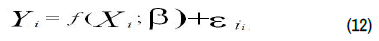
Where Yi represents the ith farm output, f (Xi; β) is a Cobb Douglas production specification, Xi is inputs vector for the ith farm and βi are the unknown parameters. Ci represents error term composed of random error Vi which has zero mean and variance N (0; σ2). Vi is associated with measurement errors and factors which a farmer does not have control over. Ui Is the other component of Ci and it is a random non-negative (Ui ≥ 0) truncated half normal N (0; σ2) variable that hinders a certain farm from achieving maximum output because it is associated with farm factors. It is associated with TE and ranges between 0 and 1. Technical efficiency is thus expressed as follows:
Where, Yi*=f(Xi; βi) was assume the highest predicted output for the ith farm.
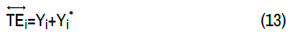
The TE of the ith farm is expressed by the ratio of the observed production output to the highest predicted output (frontier output) and expressed in equation below:

Technical inefficiency=1-TE (15)
Assessment of AE and EE: The cost frontier of the self-dual Cobb Douglas function was formulated as follows:
Ci=g (Yi, Pi; α)+Ci where Ci=1,2, ….n (16)
where Ci is the overall production cost of common bean per hectare, Yi represents the common bean output, Pi represents the cost of inputs, α represents a vector of unknown cost function parameters, and Ci is the error term formulated as Ci=Vi+Ui. Positive signs precede the error components because inefficiencies are known to raise production costs.
Economic Efficiency (EE) of the ith farm is represented by the ratio of the lowest frontier cost (C*) to the actual cost (C) as shown in equation below:
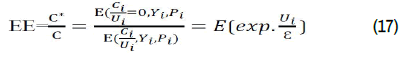
This model was run by frontier 4.1 program and it should be noted that the frontier 4.1 program estimates the Cost Efficiency (CE), Economic Efficiency (EE) is then obtained from the inverse of cost efficiency as follows:
EE=1/CE (18)
The estimation of AE can be achieved through use of efficiency results from TE an EE where EE is derived from the CE function. EE is the product of TE and AE. Hence, a measure of farm specific Allocative Efficiency (AE) is obtained from technical and economic efficiencies estimated as:
AE= EE/TE (19)
AE takes value on the interval (0,1) where 1 indicates full efficiency farm.
A variation of the Cobb-Douglas function applied in this study is the stochastic frontier model defined by J Nyoro, et al. (The Cobb-Douglas production form is chosen because its practicality and ease in the interpretation of its estimated coefficients. Despite its limitation of constant elasticity of substitution, the Cobb-Douglas is found to be an adequate representation of data.). It is simply a linearization of the above general form using logs:

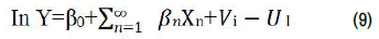
Where ln is the logarithm, the subscript, indicates the ith common bean producer household in the sample (i=1…313); ln is the natural logarithm (i.e. logarithm to base e); αn are parameters (elasticity) to be estimated (n=1….6). The parameters V and μ represents the stochastic and inefficiency components of the error terms respectively; and the other variables are as defined below. In this study, the half-normal distribution is assumed for the asymmetric technical inefficiency parameter.
The maximum likelihood estimates for the parameters of the stochastic frontier are obtained by using the Frontier 4.1 computer program, in which the variance parameters are expressed in terms of
σ2=δv2+δμ2 (21)
γ=αμ2/(αv2+αμ2) (22)
Where α2 the total variance of the model and the term is γ represents the ratio of the variance of inefficiency’s error term to the total variance of the two error terms defined above. The value of variance parameter, γ, ranges between 0 and 1.
Likelihood-Ratio (LR) statistics: In this study the gamma and the generalized Likelihood Ratio (LR) statistic are used to test for inefficiency and the appropriateness of the frontier production function (which includes on error terms) compared to the Ordinary Least Square (OLS) production function (which indicates one error terms). The gamma parameter is defined as the ratio of the variance of the one side error term μ, to total variance of the model, (γ=αμ2/α2), and the parameter is bounded between 0 and 1.
If the null hypothesis that γ equals zero is accepted. This would indicate that αμ2 is zero meaning that inefficiency effects are absent from the model. This implies that can be consistently estimated using ordinary least squares.
In this study, the LR statistic was employed to establish whether the stochastic frontier production function is preferred to the Ordinary Least Square (OLS) production function as one that the best represents the data generation process. The LR statistic was calculated as follows:
LR=-2ln(L(H0)/L(H1))=-2ln(L(H0)-lnL(H1)) (23)
Where L(H0) and L(H1) denotes the values of the likelihood function for the restricted and unrestricted frontier model, respectively.
The LR statistic has approximately a Chi-square distribution with degrees of freedom equal to the number of restrictions imposed (i.e., difference between the number of parameters estimated under H0 and H1 respectively). The null hypothesis is rejected if the computed value of LR exceeds its critical value. A significant LR statistic implies that the frontier production function fits data better than the Ordinary Least Square (OLS) production function and estimates for the farm-specific efficiencies were obtained.
Empirical model specification
Stochastic production frontier model: The model can be log linearized to be;
Where, ln denotes natural logarithm, Yi is the output in kgs per hectare, Xi are the input vectors, β0 represents intercept, β1 are unknown production function parameters, and the rest were defined earlier (Table 2).
| Variables | Measurement | Expected sign |
|---|---|---|
| Output per hectares (y) | Quintal/ha | |
| Farm size under common Bean cultivation |
Hectares | + |
| Seeds | Kg/ha | + |
| Fertilizer | Kg/ha | + |
| Labor (family and hired) | Man-days | +/- |
| Chemical inputs | Liters/ha | + |
| Oxen | Oxen-day | + |
Table 2. Variables used in the stochastic production frontier model.
Stochastic cost frontier model: The cost frontier model that would be estimated is as formulated in equation below:

Where Ci represents the total production cost per hectare, P1 represents the price of unit inputs shown in the Table 3 below;α0 represents the unknown parameter which was estimated.
| Variables | Measurement | Expected sign |
|---|---|---|
| Total production cost | ETB | |
| Land rent | ETB | + |
| Labor wage | ETB | + |
| Cost of seed | ETB | + |
| Cost of fertilizer | ETB | + |
| Cost of chemicals | ETB | + |
Table 3. Variables used in the stochastic cost frontier model.
Tobit model: A two-limit Tobit was used to determine the socioeconomic and institutional factors that influence technical, economic, and allocative efficiency as used by Ahmed. Efficiency scores lie between 0 and 1 because they are double truncated at 0 and 1 and thus form the basis to adopt the Tobit model. According to Ahmed, et al. Ordinary Least Squares (OLS) estimation method cannot be used because it gives biased estimates of parameters due to the assumption of normal distribution and homoscedasticity of the error term and the dependent variable.
The structural equation of the Tobit model is given as:
Yi*=G1β+εi (26)
Where Yi* is the latent variable for the ith common bean farm representing efficiency scores Gi represents independent variables would hypothesized to influence technical, allocative, and economic efficiency, β represents the unknown parameters, and εi is the error term with an assumption of having an independent and normal distribution with zero mean and variance (α2) (Table 4).
| Variables names | Variables codes | Measurement unit | Nature | Expected outcome |
|---|---|---|---|---|
| Age | (AGE): | Year | Categorical | + |
| Educational level of the household head | (EDUCLH): | Year | Categorical | + |
| Household size | (HHSZE): | Number of Family Member | Categorical | + |
| Sex of the household head | (SEX): | 1/0 | Dummy | + |
| Total cultivated land | (TCULTLND): | TCL | Categorical | + |
| Credit access facility | (CRDTU): | 1/0 | Dummy | + |
| Frequency of extension visit | (FEXTVST): | Number of visit | Dummy | + |
| Training | (TRAING): | 1/0 | Dummy | + |
| Crop pest | (CROPPEST) | 1 if affected, 0 otherwise | Dummy | - |
| Off/Non-farm income | OFARM | 1 if they have and 0 otherwise | Dummy | + |
| Distance from nearest market | (DISTMRKT): | Km | Categorical | - |
| Livestock holding | (LIVSTK): | Number | Continuous | + |
| Land preparation | (LANDPREP) | Number | Categorical | + |
Table 4. Variables used in Tobit model.
Variables definition and hypothesis
Definition of input and output variables in the stochastic frontier cost function model.
• Output: This is the endogenous variable in the cost
function. It is defined as the cost of inputs which is used to
produce common bean and measured in ETB during the
2020/21 production year.
• Input: Defined as the total inputs were used in the
production of common bean namely: land (Ha), labor (Man-day),
oxen (Number), fertilizers (Kg), seed (Kg) and chemicals (Li)
used during the 2020/21 production year.
Land (LAND): This represents the total physical unit of land under common bean production in hectare. This was hypothesized that households which have a wide land will get more production of common bean. This suggests that the more farm land a farmer allocated to bean farming, the higher the yields obtained, which presents similar findings as those reported by Goni et al. The authors argued that most smallholder farmers usually fail to maximize bean yields due to underutilization of farm land. This might be due to limited availability of other production factors or due to farmer's risk averseness coupled with rainfall fluctuations 57 brought about by climate change. However, Ugwumbain Nigeria observed that land was underutilized mainly due to land tenure problems associated with land fragmentation. Therefore based on the results it is implied that as the sizes of land holding continue to decline, it is increasingly going to become difficult to increase productivity through expansion in plot sizes.
Human labor (LABOR): Represents the total human labor employed in the production process. It was measured in man days (equal to eight hour per day). So the family which has many labor forces will get more common bean production. A positive influence was also reported by Aboki et al.; Ayinde et al.,; Girei et al., and Ahmed et al., explained that many farmers depend on household labor to increase production due to its availability, inexpensiveness, and ease of timely allocation in different farm activities especially during planting, weeding, and harvesting.
Oxen power (OXEN): Oxen powers were measured using the total amount of oxen days allocated for ploughing and hoeing activities of common bean production. It was measured in oxen-days (one oxen-day is equivalent to eight working hours). Thus, possessing a large number of oxen is crucial to increase EE in crop production in the study areas. This result is consistent with the findings of Endrias et al., on maize efficiency.
Fertilizer (DAP): The total amount of DAP (in Kg) used in common bean production during the 2020/21 production year. This would have positive effect on the production of common bean. This suggests that increasing the amount of planting fertilizer used would contribute to higher bean yields in the area by a factor of 10. The results are consistent as hypothesized and they reflect the findings presented by Tchale, in Malawi where fertilizer was a key factor in production of major crops grown by smallholder farmers. Reardon et al., also found a positive effect of fertilizer on productivity in case studies from Burkina Faso, Senegal, Rwanda and Zimbabwe. However, the findings contradict who observed that soils in Uganda were fertile enough and could produce relatively high yields even without adequate fertilizer use. As such, from the results it is evident that to achieve higher bean productivity, farmers in Eastern Uganda need to increase their usage of planting fertilizer.
Seed (SEED): Represents the type of common bean seed quantity used by the ith household. It was included in the production frontier function in physical quantity and measured in kg. This would be hypothesized positive effect. This suggests that planting more seeds improved bean productivity significantly, which is attributed to the fact that the increased number of seeds per hole helped reduce the risk of plants failing to sprout and translated into higher production from a unit piece of land. Given that seed had the largest elasticity; it might also imply that seed was the major limiting factor of production that constrained common bean farmers from maximizing their output. The importance of seeds in determining productivity has also been emphasized by Reardon et al.
Chemicals (CHEM): This is a physical quantity of chemicals such as insecticides and pesticides applied by the sample households for protection of insects and pests in common bean production, respectively. It was measured in liters and its monetary value.
Given the above-specified input variables, the functional relationship between inputs and output used in the cost function can be specified as follows:

Where,
Ci=Total cost of the ith farm (qt)
f(.)=appropriate functional form
(e.g. Cobb-Douglas)
βi=vector of unknown parameters to be
estimated;
εi=composed error term (εi=Vi+Ui),
Vi=a disturbance term
which accounts for factors outside the control of the farmer
Ui=non-negative
random variable which captures the technical inefficiency
in production.
The linear functional form of Cobb-Douglas production function used for this study is given as:

Efficiency factors of common bean production and the working hypothesis.
Dependent variables: The dependent variables for this study were: TE, AE and EE scores of common bean production obtain from SFPF. Independent variables had identified based on theory and previous studies on production and factors affecting efficiency of production, the following variables expected to determine efficiency differences among common bean producers.
Age of the household head (AGE): It is a categorical variable which refers to the age of the household head measured in years. Therefore, in this study age of the household head was hypothesized to have positive effect on efficiency. This means that older farmers were less technically efficient in bean production than their younger counterparts consistent with findings by Kibaara, in Kenya. The finding is attributed to the fact that older bean farmers in the study area are relatively more reluctant to take up better technologies, instead they prefer to hold to the traditional farming methods thus become more technically inefficient compared to their younger counterparts. This reluctance to embrace innovative farming methods is also responsible for the constant returns to scale realized earlier. However, Illukpitiya, found contradicting results in Sri-lanka; where it was observed that elderly farmers had a wealth of experience and were technically more efficient in production than their younger counterparts. The inconsistency may be due to differences in socio-economic characteristics of the sampled farmers, however, it is important to emphasize that being older may not always substitute being more experienced.
Educational level of the household head (EDUCLH): It was the categorical variable, which was measured by level of schooling attaining. Education increases the ability to get, process, and use information. The significant effect of education on AE confirms the importance of education in increasing the efficiency of common bean production. The result indicates that, AE require better knowledge and managerial skill than TE and EE. In other words, educated households have relatively better capacity for optimal allocation of inputs. In line with this study, research done by Aynalem, in North Ethiopia, Keinde and Awoyemi, and Ogundari and Ojo, both in Nigeria and Kifle, have also found education to influence AE positively and significantly.
Household size (HHSZE): A household is an important source of labor supply in rural areas. It is expected that households with many members have better advantage of being able to use labor resources at the right time, particularly during peak cultivation periods. Therefore, household size could have positive effect in raising the farmer’s production efficiency. However, it is important to evaluate whether relatively large households are more efficient than small ones.
Following Coelli it hypothesized that relatively large households in the area will expect to be more efficient than small-sized households. A positive influence was also reported by Aboki. Ayinde and Ahmed explained that many farmers depend on household labor to increase production due to its availability, inexpensiveness, and ease of timely allocation in different farm activities especially during planting, weeding, and harvesting.
Sex of the household head (SEX): This is a dummy variable that is measured as 1 if the household head is male and 0, otherwise. Therefore, it hypothesized that female-headed households are expected to be less efficient than their male counter parts. The implication is those female households headed are the one who were responsible for many household domestic activities such as collecting of fire wood from the field, fetching water from the far distant rivers, childrearing and household management obligations and also probably use inputs fewer than male household heads. This result is consistent with Aynalem.
Land/farm size: This refers to the area of cultivated land (own, rented) for common bean by the household during 2020/21 production year. According to Andreu, larger farms are relatively better efficient than small size farms. Therefore, households with larger area of cultivated land for common bean had the capacity to use compatible technologies that could increase the efficiency of the household, enjoy economies of scale and relatively better efficient than small size farms.
Credit access (CREDIT): This is a dummy variable that represents the use of credit for farm related purposes by farmers. The actual amount of credit received used 1 and 0, otherwise. Since credit utilized is an important source of financing the agricultural activities of small holder farmers Okoye et al. It was hypothesized that households who have utilized to credit sources were more efficient than others. Farmers who borrowed agricultural credit have higher EE than those who did not acquire credit. Ahmed also found credit access being a positive determinant of EE. Sibiko explained that farmers who borrow money for agricultural production afford the yield-improving inputs such as improved seeds and fertilizers, and labor-saving inputs such as herbicides. This increases their yield while reducing some production costs, which translates to increased productivity and profitability.
Frequency of extension visit (FEXTVST): Frequency of extension visits is a dummy variable and medium for the diffusion of new technologies among farmers and hence improves the efficiency of farmers. Therefore, extension visit expected to have a positive effect on efficiency.
Frequency training on common bean production (FTCOMBP): This is a dummy variable that represents the access to training for farm related activities. If the household has got training, the variable takes a value of 1 and 0, otherwise. So, households who receive training service had been hypothesized to be more efficient than those who did not receive training.
Crop pest: It was taken as dummy variable, which takes 1 if the farmer’s common bean were exposed to crop pest and 0 otherwise.
There are different types of crop pest affects common bean in study area. From those, the well-known were Bean stem maggot and African bollworm. Bean stem maggot: Larvae feed on the outer tissue of the stem at ground level. This causes longitudinal cracks, yellowing of the leaves and weak and stunted plants. Bean seedlings can die. Bean stem maggot can be controlled with early planting, crop rotation, using tolerant varieties or dressing seed with systemic insecticides whereas, African bollworm is a caterpillar that bores pods, making clean round holes in the pods. Regularly monitor the crop, and handpick and destroy infested pods and the bollworms. When fields are large or when there is a heavy infestation. So, this crop pest has adverse effect on economic efficiency level of common bean producer. If the sample common bean producer is affected by pest, obviously there would be a loss in output of common bean production. Because of this, pest was expected to affect efficiency level of smallholder common bean production negatively.
Off/non-farm income (OFARM): This was treated as a dummy variable and measured as 1 if the household is involved in off/non-farm activities and, 0 otherwise. Farmers engaged in off/non-farm income were expected to generate more income. Farmer engaged in off/non-farm activities was more efficient than his counterpart, because the income obtained could be used for the purchase of agricultural inputs and augments financing of household expenditures which would entirely dependent on agriculture. Therefore, it was hypothesized that farmers who engage in off/non-farm income were expected to have a positive effect on efficiency.
Distance from the market (DSTMRKT): It is the categorical variable defined as the distance for common bean producer households from the nearest market and measured in km of single trip. This variable is proxy to transportation cost, loss cost, and marketing cost. Being far from home to the nearest market is another indicator of market isolation. Those households who are close to the nearest market are encouraged to have better probability of supplying their common bean to the market by increasing volume of common bean production. It was expected that longer distance increase travel time and travel cost, which affects the common bean production negatively due to adverse impact on market participation. Abraham indicated that distance to market caused market surplus of cabbage to decline. Therefore, distance to the nearest market center was hypothesized to negatively associate with common bean economic efficiency.
Livestock holding (LIVSTK): This is the total number of livestock owned in terms of tropical livestock unit. Livestock could support crop production in many ways; they can be source of cash, draft power and manure that will be used to maintain soil fertility. Therefore, in this study the effect of livestock on efficiency was hypothesized to be positive. As in the case of Aynalem, confirms the considerable contribution of livestock in reducing the current cost of inputs in common bean production as source of draft power, food, income, for inputs purchase and organic fertilizers.
Therefore, in this study the effect of livestock on efficiency would be hypothesized to be positive (Table 5).
| Variables names | Variables codes | Measurement unit | Nature | Expected outcome |
|---|---|---|---|---|
| Age | (AGE): | Year | Categorical | + |
| Educational level of the household head | (EDUCLH): | Year | Categorical | + |
| Household size | (HHSZE): | Number | Categorical | + |
| Sex of the household head | (SEX): | 1 if male and 0 if female | Dummy | + |
| Land/farm size | (LNDSIZE): | Ha | Categorical | + |
| Credit access facility | (CRDTU): | 1/0 | Dummy | + |
| Frequency of extension visit | (FEXTVST): | 1 if they have got and 0, otherwise | Dummy | + |
| Training | (TRAING): | 1/0 | Dummy | + |
| Disease occurrence | (DISOCC) | 1 if there is, 0 otherwise | Dummy | + |
| Off/non-farm income | OFARM | 1 if they have and 0 otherwise | Dummy | + |
| Distance from nearest market | (DISTMRKT): | Km | Categorical | - |
| Livestock holding | (LIVSTK): | Number | Continuous | + |
| Land preparation | (LANDPREP) | Number | Categorical | + |
Table 5. Hypothesis and definition of variables for the common bean production summary.
Results and Discussion
This chapter presents the descriptive results of socio-economic characteristics and farm specific factors of production of sample households. It also provides the empirical results of Tobit two-limit model for technical, allocative and economic efficiency of common bean production with detailed explanation of significance variables.
The results of descriptive analysis
Demographic, socio-economic and institutional characteristics of the sample households: For the descriptive statistics such as mean, percentage, standard deviation and frequency were used.
Age: Regarding to common bean production, age of the household head was believed to be a great source of experience in day-to-day activity of human being. So, elderly heads of household were expected to have more experience in common bean production. As a result in Table 6, the average age of the sample household heads was 45.4 years with maximum of 66 and minimum of 29 years. Of the total sample farmers, nearly 7.7% were younger than 35 years and only about 3.51% were older than 58 years and were above economically active range. The majority of the household heads (51.11%) were found in the age ranges of 36 and 46 years.
Family size (FAMSIZE): The family size of the respondents was categorized into four. As (Table 6) below reveals respondents with family size of the sample farmers ranged from one (1) to 13 with a mean of 10.25. The majority of the households (47.3%) had 11-15 family members whereas, 46% of sample households had 7-10 family members and 6.4% had 3-6 also 0.3% had 16 family members.
Educational level (EDUC): Education was a social capital which has a positive influence on household ability to understand to utilize new technological information and also to know their right and obligation. The survey result showed that from the sampled respondents of smallholder farmers, only 46.6% of the household heads were illiterate while the remaining 53.4% of the respondents were at least capable of reading and writing. As indicated in Table 6, out of the total sample household heads, 33.6% have attained formal education while 16.3% of them were able to read and write and 3.5% of the respondent attended the religious education.
Marital status of the sample household heads: Regarding the marital status of respondents as indicated in Table 6 below, 92% of the sample households were married households. The result also revealed that 1.6% of the sample households have never married and 6.4% were divorced and non-of them were widowed.
Religion of sample household heads: Religion of sample household heads about 55% of the sample farmers selected for this study were followers of Orthodox, 36.7% of the sample farmers were followers of Protestant and 8.3% were Muslim as shown in Table 6 below.
Land/farm size: This refers to the area of cultivated land (own, rented) for common bean by the household during 2020/21 production year. According to Andreu, larger farms are relatively better efficient than small size farms. Therefore, households with larger area of cultivated land had the capacity to use compatible technologies that could increase the efficiency of the household, enjoy economies of scale and relatively better efficient than small size farms. According to the survey result, the average land holding of the sample households was 1.54 hectare with a standard deviation of 1.09 and minimum of 0.25 hectare and maximum of 3.5 hectare.
Extension service: It is a dummy variable, in order to give effective extension service to the farmers, the district assigned professional development agents in each kebele. The development agents are graduates of different colleges specializing in three agricultural streams such as crop production, animal husbandry and natural resource management. In this study, 92.3 percent of the sample respondents reported that they have been receiving extension services and advice about common bean production. The extension workers also visit farmers on different intervals. Some farmers are being visited more frequently while others have no chance at all to be visited by extension workers. The survey result indicates that, about 59.4, 18.6, 11.8 and 2.5 percent of the sample households were received extension service more than four times (year), three times (year), two times (year) and one times (year) respectively.
Land preparation: The number of ploughing indicates an intensity of land preparation that helps for appropriate germination of the seed which is expected to have a direct impact on yield.
As indicated in Table 6 below, about 32.90% of the respondents ploughed their farm one times, 61.66% ploughed their farm two times and 5.44% of the farmers plough their land three times.
Distance to nearest market: This variable represents the distance between a household residence and the nearest market center measured in km. It was hypothesized that distance from market place is negatively related to efficiency. This was because those farmers far away from market are less accessible for farm inputs and market information and transportation become costly and difficult. Out of the total sample households surveyed, about 49.52% indicated that their common bean farm was inside the range of 2 km-4 km from the market and 36.42% were even inside the radius of 5 km-7 km where as 14.06% were far from the home above 8 km.
| Category | Value | ||
|---|---|---|---|
| Number | Percent | ||
| Age | 29-35 | 24 | 7.7 |
| 36-46 | 160 | 51.1 | |
| 47-57 | 118 | 37.7 | |
| 58 and above | 11 | 3.5 | |
| Total | 313 | 100 | |
| Mean | 45.395 | ||
| Std. deviation | 6.553 | ||
| Family size | 3-6 | 20 | 6.4 |
| 7-10 | 144 | 46 | |
| 11-15 | 148 | 47.3 | |
| Above 16 | 1 | 0.3 | |
| Total | 313 | ||
| Mean | 10.29 | ||
| Std. deviation | 2.19 | ||
| Education | Illiterate | 146 | 46.6 |
| Read and write | 51 | 16.3 | |
| 1-5 grade | 105 | 33.6 | |
| Grade 6 and above | 11 | 3.5 | |
| Total | 313 | ||
| Mean | 3.5 | ||
| Std. deviation | 1.27 | ||
| Land size | < a half hectare | 32 | 10.22 |
| A Half hectare | 93 | 29.71 | |
| > a half hectare | 208 | 60.07 | |
| Total | 313 | ||
| Mean | 1.54 | ||
| Sta. deviation | 1.09 | ||
| Land preparation | One time ploughing | 103 | 32.9 |
| Two time ploughing | 193 | 61.66 | |
| Three time ploughing | 17 | 5.44 | |
| Total | 313 | ||
| Mean | 2.09 | ||
| Sta. deviation | 1.89 | ||
| Distance from market | 2-4 km | 155 | 49.52 |
| 5-7 km | 114 | 36.42 | |
| Above 8 km | 44 | 14.06 | |
| Total | 313 | ||
| Mean | 4.94 | ||
| Sta. deviation | 2.39 | ||
| Source: Computed from field survey data, 2021 | |||
Table 6. Socio-economic and institutional characteristics of the households (categorical variable).
Sex: The sample composed of both male and female smallholder farmers. Of the total sampled smallholder farmers, 3.6% or 11 were female and 96.4% or 302 were male.
Access to credit: Common bean requires high costs for production. Respondents in the study area interviewed whether or not they need access for credit services. From the total respondents replied about 72.21 percent were not get credit service and 27.79 percent were got credit service in the institute as present in Table 7. Mostly smallholder farmers, get credit from creditors (private lenders), Omo-microfinace institute and bank. The study indicated that in the district 5.38 percent of credit had gain from private lenders with interest rate reached 50 up to 100 percent, 18.47 percent from Omo-microfinance with interest rate 300 ETB from 1000 ETB in a year and 3.93 from commercial bank of Ethiopia with interest rate of 100 ETB from 1000 in a month.
Extension service: In order to give effective extension service to the farmers, the district assigned professional development agents in each kebele. The development agents are graduates of different colleges specializing in three agricultural streams such as crop production, animal husbandry and natural resource management. In this study, 92.3 percent of the sample respondents reported that they have been receiving extension services and advice about common bean production. 7.7% of the respondent’s haven’t got extension service. The extension workers also visit farmers on different intervals. Some farmers are being visited more frequently while others have no chance at all to be visited by extension workers. The survey result indicates that, about 59.4, 18.6, 11.8 and 2.5 percent of the sample households were received extension service more than four times (year), three times (year), two times (year) and one times (year) respectively as show in Table 7.
Training: An appropriate training given to the farmers may improve productivity by enhancing their management capacity and their production performance. In this study area, farmers were getting training from surrounding agricultural office and other governmental and non-governmental organizations. Among the sample farmers, 93.7 percent of farmers were trained on different common bean related aspects and the rest 6.3 percent of the respondent had not received any training on the subject matter previously. This indicates that majority of the sample farmers were received training as shown in Table 7.
Crop pest: It was taken as dummy variable, which takes 1 if pest affect the product of common bean and 0 otherwise. In the study area common bean production is sensitive to crop pest. Crop pest has adverse effect on economic efficiency level of common bean producer. If the sample common bean producer is affected by crop pest, obviously there would be a loss in output of common bean production. Because of this, crop pest was expected to affect efficiency level of smallholder common bean production negatively. Among the sample farmers, 37.8 percent of farmers were exposed to common bean crop pest and the rest 62.2 percent of the respondent had not expose to common bean crop pest. This indicates that majority of the sample farmers common bean was not exposed to crop pest as shown in Table 7.
Off/non-farm income (OFARM): This was treated as a dummy variable and measured as 1 if the household is involved in off/non-farm activities and, 0 otherwise. Some farmers in the study area were engaged in various off/non-farm activities. The main activities were selling of firewood, being hired in other’s farm and selling local drink. The survey indicated that 11.11% of the respondents were engaged in off/non-farm activities. They also mentioned that availability of excess labor, attractive income and mainly shortage of land as the reasons for their engagement in off/non-farm activates.
| Variables | Number | Percent | |
|---|---|---|---|
| Sex | Male | 302 | 96.4 |
| Female | 11 | 3.6 | |
| Access to credit | Yes | 87 | 27.79 |
| No | 226 | 72.21 | |
| Extension contact | Yes | 289 | 92.3 |
| No | 24 | 7.7 | |
| Training | Yes | 293 | 93.7 |
| No | 20 | 6.3 | |
| Crop pest | Yes | 118 | 37.8 |
| No | 195 | 62.2 | |
| Off-farm income | Yes | 66 | 11.11 |
| No | 247 | 88.89 | |
| Source: Computed from field survey data, 2021 | |||
Table 7. Socio-economic and institutional characteristics of the households (dummy variable).
Livestock holding: Livestock have diverse function and livestock plays crucial roles for the livelihood of the farmers in mixed farming system. They provide food in the form of meat, milk, and non-food items such as draft power and manure as inputs into crop production. As shown in Table 8, goat and sheep, hen, oxen, cows, calves and donkey are the livestock which the respondents have. On average, the sample household farmers owned 7.05, 6.3, 2, 1.75, 1.27, and 1.11 respectively. Donkey was use for transport of farm inputs and outputs. Moreover, the sample respondent owned 7.05 sheep and goats were keep as a source of income and hedging against risk during the crop failure. Moreover, the survey results showed that the average tropical livestock unit per sample household was 4.78 per household with the standard deviation of 2.75 TLU. On top of this, as it is indicated in Table 8, the average holding of oxen per household found to be 1.92 TLU which statically implies that 2 oxen per household sample respondent with a standard deviation of 0.92 TLU. The standard deviation here indicates that there is variability in livestock holding among the households.
Cropping system: The dominant farming system of the district is crop-livestock mixed. Crop production district is limited to autumn season and the major types of crop that are produced include common bean, teff, wheat, maize, barley, and sorghum. The district was experienced by producing twice a year. The first season was start from February up to the end of July and the second start from the mid of August up to the end of December. On the first season the most growing crops are teff, maize, wheat, barley, sorghum and common bean in small amount. On the second season most of the land i.e. on average almost half the total hectare will covered by common bean. Though modern input application, especially fertilizer is there, the performance of major crops in terms of yield is encouraging. The mean area coverage (hectare) of major crops in 2020/21 production year is presented in Table 8. The result indicated that on average sample farmers have of 0.25 with the minimum and maximum of 5.5 hectare. As shown in Table 8, in the district most farmers use their own land for the production of common bean on average 1.54 hectare of land with the standard deviation of 1.09 because the data was collected in second season Which implies that common bean is the most dominant legume crop in the district as compared to other cereals such as wheat, teff, maize, barley and sorghum.
| Livestock | Mean | Std. dev. | Min | Max |
|---|---|---|---|---|
| Oxen | 1.92 | 0.92 | 0 | 5 |
| Cow | 1.27 | 0.81 | 0 | 4 |
| Calf | 1.03 | 0.7 | 0 | 4 |
| Adult goat and sheep | 2.49 | 2.44 | 0 | 12 |
| Goat and sheep | 4.56 | 3.78 | 0 | 18 |
| Donkey | 1.11 | 0.84 | 0 | 3 |
| Hens | 6.3 | 5.63 | 0 | 25 |
| TLU | 4.78 | 3.11 | 0.38 | 15.06 |
|
|
||||
| Common bean | 1.54 | 1.09 | 0.25 | 5.5 |
| Teff | 0.95 | 0.95 | 0.05 | 1.5 |
| Wheat | 0.4 | 0.58 | 0 | 1.5 |
| Maize | 0.5 | 0.89 | 0.025 | 1.5 |
| Barley | 0.15 | 0.39 | 0 | 0.25 |
| Sorghum | 0.05 | 0.14 | 0 | 0.08 |
| Total | 3.59 | |||
| Source: Own survey (2021) | ||||
Table 8. Socio-economic characteristics of the sample households (continuous variable).
Inputs and input costs: Table 9 presents the description of inputs, their mean, min, max and associated costs. The total amounts of DAP fertilizer measured in Kg while its costs were expressed in Ethiopian Birr (ETB). On average, 239.13 kg of DAP was used while the average cost of these inputs was 5021.73 ETB.
The size of land used for common bean in study area by each farmer was measured in hectare. On average, the rental value of good quality of land 4424 ETB per hectare for one production year was used to estimate cost of land. Accordingly, on average, a given household allocate a total of 1.54 hectare of land for common bean production and its average cost was computed as 6812.96 ETB. On average, about 2.96 liter of chemicals was used during the production of the common bean and its average associated cost was 296.16 ETB.
The total amount of seeds used was computed as the sum of the seed. The corresponding seed costs were computed as the product of the total amount of seed used and market prices of a unit kg of seed. On average, the amounts of seed were 63.37 kg of common bean per household head of the respondent. The associated average costs of common bean seed 1550.26.
Labor was aggregated for each farmer in single unit man/days. The cost of hired labor was estimated based on the daily average wage rate (80 ETB per day) of the nearly village. As a result, total cost of labor input was the sum of cost of hired labor and opportunity cost of family labor. In aggregate, the average use of labor in man/days equivalent was about 105 which statically imply that 105 labor and labor costs has an average of 8436 ETB.
| Variables | Unit | Mean | Std. dev. | Min. | Max. |
|---|---|---|---|---|---|
| Output | Quintal | 23.2 | 11.8 | 4 | 45 |
| Quantity of common bean seed | Kg | 63.75 | 39.78 | 25 | 250 |
| Labor (family and hired) | Man/days | 105.45 | 42.86 | 20 | 226 |
| Fertilizer (DAP) | Kg | 239.13 | 124.46 | 50 | 600 |
| Quantity of chemical | Liter | 2.96 | 0.88 | 1 | 5 |
| Land | Hectare | 2.4 | 1.45 | 0.25 | 5.5 |
| Total cost of output | ETB | 25377.67 | 11567.31 | 5360 | 66749 |
| Cost of seed | ETB | 1550.26 | 40.32 | 304 | 3737 |
| Cost of land | ETB | 6812.96 | 2533.71 | 1106 | 24332 |
| Cost of DAP | ETB | 5021.73 | 1384.23 | 1050 | 12600 |
| Cost of labor | ETB | 8436 | 428.64 | 1600 | 18080 |
| Cost of oxen | ETB | 3260.56 | 1765.33 | 1200 | 7500 |
| Cost of chemicals | ETB | 296.16 | 88.35 | 100 | 500 |
Table 9. Input uses and outputs for common bean production in district with its costs.
Table 9 result represents the main inputs uses for the production of common bean. The responses of household respondents show cost of land, chemical and fertilizer (DAP) were widely used for common bean production. From the Table 9, from the respondent, 24 households (7.66%) were rented the land for common bean production, also 309 households (98.72%), farmers were use chemical and 310 households (99.04) farmers were used fertilizer (DAP) and the source of the inputs are agricultural office, cooperative and trader. As shown in Table 10 the response of household shows all most all farmers use fertilizer (DAP). Field chemicals include pesticides and insecticides.
| Input factor | Response | Frequency | Percent |
|---|---|---|---|
| Land rented | Yes | 24 | 7.66 |
| Pesticide/chemical | Yes | 309 | 98.72 |
| Fertilizer (DAP) | Yes | 310 | 99.04 |
|
|
|
|
|
| Agricultural office | Yes | 206 | 65.81 |
| Cooperative | Yes | 103 | 32.92 |
| Trader | Yes | 4 | 1.27 |
| Source: Own survey (2021) | |||
Table 10. Proportion of input user households in 2020/21 production year.
Production constraints: Crop pest was a serious problem that farmers were facing in the study area. About 38.0% of respondents reported that they were facing crop pest whereas 29.4% believes crop disease was the problem that they were facing. In addition to this, there was also a wide range of weed infestation in the study area which accounts 26.2%. Farmers also reported that there was labor shortage during peak agricultural production seasons (Table 11).
| Production problems | Number of farmers | Percent |
|---|---|---|
| Weed infestation | 82 | 26.2 |
| Crop disease | 92 | 29.4 |
| Crop pest | 119 | 36.7 |
| Seed shortage | 18 | 5.8 |
| Shortage of draft animal | 2 | 0.6 |
| Total | 313 | 100 |
Table 11. Agricultural production constraints.
Descriptive statistics of variables used in the model: This section present summary statistics results of production variables used for analysis in the stochastic production frontier model, cost frontier and in Tobit model.
Descriptive s tatistics of production function variables: On average, sample farmers obtained 23.2 quintal of common bean. The average land area allocated to common bean production (owned shared and rented land) by household was 1.54 ha and ranged from 0.25 ha to 5.5 ha. The amount of seed that sampled households used were 63.75 kg on average. Like other inputs, human labor and oxen power inputs were also important, given a traditional farming system in the study area. Sampled households on average used 105 man equivalent labor and 14.3 oxen days for the production of common bean during 2020/21 production of second season. Sample farmer households also on average used 239.13 kg of DA (Table 12).
| Variable | Mean | Std. dev. | Min. | Max. |
|---|---|---|---|---|
| Output (qt) | 23.2 | 11.8 | 4 | 45 |
| DAP (kg) | 239.13 | 124.46 | 50 | 600 |
| Oxen (OD) | 14.3 | 7.3 | 6 | 22 |
| Seed (kg) | 63.75 | 0.4 | 25 | 250 |
| Labor (MD) | 20 | 4.3 | 10 | 29 |
| Land (ha) | 1.54 | 1.09 | 0.25 | 5.5 |
| Source: Own survey (2021) | ||||
Table 12. Summary of input-output variables used to estimate the production function.
Descriptive statistics of variables used to estimate the cost function: As presented in Table 13 the mean and standard deviation of each variable used in the cost function along with their involvement to the total cost of cultivation are discussed as follows. On average total cost of Birr 25377.67 was required to produce 23.2 quintal of common bean. Among the various factors of production, the cost of labor, land and DAP accounted for the highest share 8436, 6812.96 and 5021.73 respectively. From the following the cost of oxen, cost of seed, and cost of chemicals takes, 3260.56, 1550.26, and 296.16 respectively out of total cost of cultivation.
| Variables | Unit | Mean | Std. deviation | Percentage share of total cost |
|---|---|---|---|---|
| OUTPUT | Quintal | 23.2 | 11.8 | - |
| Total cost of output Birr | 25377.67 | 11567.31 | - | |
| Cost of seed | Birr | 1550.26 | 40.32 | 6.18 |
| Cost of land | Birr | 6812.96 | 2533.71 | 26.84 |
| Cost of DAP | Birr | 5021.73 | 1384.23 | 19.78 |
| Cost of labor | Birr | 8436 | 428.64 | 33.24 |
| Cost of oxen | Birr | 3260.56 | 1765.33 | 33.24 |
| Cost of chemicals | Birr | 296.16 | 88.35 | 1.16 |
Table 13. Descriptive statistics of variables used to estimate the cost function.
Summary of descriptive statistics of efficiency model variables: As presented in Table 14 the mean and standard deviation of each variable used in efficiency model. On average the age composition of the household was 45.4 with standard deviation of 6.55 and the family size was 10.29 with standard deviation of 2.19. The education also takes 3.5 mean grade of the household with the standard deviation of 1.27. The land size which common bean produced was counts of 1.54 mean of hectare with the standard deviation of 1.09 and land preparation also 2.09 of mean value with standard deviation of 1.83. Among the various factors of production, the distance from the market counts 4.94 km from farm land with standard deviation of 2.39. The total livestock unit also takes the value of 4.78 of mean and standard deviation of 3.11.
Sampled households, on average, 96.4% of them were males household and rests were females. Out of the total respondents, 27.79% of them reported that they had an access to credit for common bean production during the survey period. From the sampled households, on average 92.3 get the extension contact by different frequency and the rest 7.7% wouldn’t get. Out of the sampled households, 37.8% were affected by the crop pest and 62.2% of them were able to control it. Only about 11.11% of the sampled farmers reported to earn off/non-farm income (Table 15).
| Variables | Mean | Std. dev. |
|---|---|---|
| Age | 45.4 | 6.55 |
| Family size | 10.29 | 2.19 |
| Education | 4.5 | 1.27 |
| Land size | 1.54 | 1.09 |
| Land preparation | 2.09 | 1.83 |
| Distance from market | 4.94 | 2.39 |
| TLU | 4.78 | 3.11 |
| Source: Own computation (2021) | ||
Table 14. Descriptive statistics of categorical and continuous variables used to estimate efficiency of common bean.
| Variables | Percent of Dummy | |
|---|---|---|
| Dummy=1 | Dummy=0 | |
| Sex | 96.4 | 3.6 |
| Access to credit | 27.79 | 72.21 |
| Extension contact | 92.3 | 7.7 |
| Training | 93.7 | 6.7 |
| Crop-pest | 37.8 | 62.2 |
| Off-farm income | 11.11 | 88.89 |
| Source: Own computation (2021) | ||
Table 15. Descriptive statistics of dummy variables used to estimate efficiency of common bean.
Econometric results
This section presents the econometric model outputs of the production function; efficiency scores and factor that affect technical, allocative and economic efficiency of smallholder farmers in common bean production in the study area.
Hypothesis testing/estimation of product frontier: Before running the econometric model, first check the multicollinearity test in between continuous and dummy variables by using Variance Inflation Factor (VIF) and contingency coefficient. Second Cobb-Douglas versus Tran slog production function was check by using the decision to select functional form depends on the calculated (generalized) likelihood ration. The Third OLS versus Maximum Likelihood Estimation (MLE) or Stochastic Frontier Model (SFM) was checked by log likelihood ration. The test of each variables and models are shown below one by one.
The first conducted was the existence of multicollinearity problem between continuous and dummy variables. According to Gujarati, the value of VIF more than 10 is usually considered as an indicator of serious multicollinearity, and should be excluded from the model. On the other hand, variables having VIF of less than 10 are believed to have no serious multicollinearity problem and able to include as explanatory variables in the model. According to Gujarati, VIF is defined as:
VIF (Xi)=(1/(1-R2)) (29)
Where, xi=the ith explanatory variable regressed on the other explanatory variables.
R2=adjusted R-square; the coefficient of the determination in the (auxiliary) regression of Xi on the remaining repressors
As shown in Appendix Table 1-3 VIF means the farm specific variables, VIF of the explanatory cost of variables and VIF for the continuous socio-economic variables was 3.1, 5.93, and 1.34 respectively. This implies that there is no multicollinearity problem among the variables because of the number or the value of VIF is less than 10.
The contingency coefficients are calculated for each pair of discrete variables using contingency coefficient test.
C=√χ2/n+χ2 (30)
Where, C=contingency coefficients; n=total sample size; χ2=Chi-square test
As shown in the appendix Table 4 results of the contingency coefficient test such as, the categorical or dummy variables, contingency coefficient, which is a chi-square based measure of association, was employed to check for the presence of multicollinearity. According to Gujarati, a contingency coefficient value of 0.75 and above (i.e. ≥ 0.75) indicates the existence of strong relationship between the variables. By looking the contents of the table, it can be concluded that there is no problem of association among the variables as the respective coefficients are very low. Consequently, all the discrete variables were included in the estimation of the specific multiple linear regression models.
The second hypothesis tested was whether the problem technology of the sample household is better represent by the Cobb-Douglas function or Translog production function. To select the appropriate specification, both Cobb-Douglas and Translog function forms were estimated at shown on Appendix Table 5. The null hypothesis is the coefficient of interaction and square terms of Translog production function are zero. Based on equation 23 the result shown in Table 5 indicates that the calculated Likelihood Ration value (LR) equal to 28.14 that means LR=-2(lnH0)-ln(H1)=-2(-34.7-(-20.64)=-2*(-14.7)=28.14 while the critical likelihood ratio value at 21 degree of freedom equal to 32.67 (tabulated) or the critical value at (5%,1) is 32.67. since the calculated LR value is less than the critical value of Chi-square at 21 degree of freedom, the null hypothesis is accepted at 1% level of significance implying that Cobb-Douglas function form adequately represents the input output data of common bean production.
The third hypothesis tested was whether Stochastic Frontier Models (SFM) adequately represents the input output data of common bean production or not. In other word, whether technical, allocative, and economic inefficiency is present in common bean production or not was tested. The test was conducted based on the statistical significance of standard deviation of technical inefficiency. The result of the test helps to identify whether common bean producer farmers are technically efficient or not. This is made in order to decide whether the traditional average production function (OLS) best fits the data set as compared to Stochastic Frontier Model (SFM) selected for this study. That mean if the null hypothesis H0:γ=0 is accepted against alternative hypothesis H1: γ ≠ 0, then the Stochastic Frontier Models (SFM) is identical to OLS specific indicating that there is no inefficiency problem within the common bean producer sample households. The result based on the equation 23 (Table 15) below indicates that calculated likelihood ratio value LR equals to 85.82 while the critical chi-square value at 5% level of significance equals to 3.84. Since the calculated likelihood ratio value LR is greater than the critical value of chi-square (χ2) at 1 degree of freedom, the null hypothesis is not accepted at 5% level of significance implying that stochastic production frontier model is appropriate than OLS or there is significant technical inefficiency variation among sample household farmers.
The fourth hypothesis tested was whether the explanatory variables/socio-economic variables in technical inefficiency effect model are simultaneously equal to zero or not. By using equation 23 (LR) the result shows below in table 24 indicates that the calculated value of LR equals to 85.82 while the critical chi-square (χ2) at 13 degree of freedom at 5% level of significance equals to 22.36. Since the calculated Likelihood Ratio value (LR) is greater than the critical chi-square (χ2) value the null hypothesis that explanatory variables in the technical inefficiency effect model are simultaneously equal to zero was not accepted at 5% level of significance. Hence, the explanatory variables associated with technical inefficiency effect model are jointly different from zero or jointly explain technical efficiency differences among sample common bean producer farmers (Table 16).
| Null hypothesis | Degree of freedom | LR value | χ2 at 5% value | Decision |
|---|---|---|---|---|
| H0; γ=0 | 1 | 85.82 | 3.84 | Not accept H0 |
| H0; δ0=δ13=0 | 13 | 85.82 | 22.36 | Not accept H0 |
| H0;β7=...β27=0 | 21 | 28.14 | 32.67 | Accept H0 |
| Source: Own computation | ||||
Table 16. Likelihood ratio tests for the model and parameters of the stochastic frontier analysis.
Production and cost efficiencies of farm specific variables: The Maximum-Likelihood (ML) estimates of the parameters of the stochastic production frontier were obtained using the program FRONTIER 4.1 software. These results were present in Table 17, which also presents the OLS results of the average production function for comparison. The sign of the slope coefficients both OLS and ML estimates are positive. The estimate of variance parameter gamma is also significantly different from zero, which implies that the inefficiency effects are significant in determining the level of common bean production and output of the sampled household farmers. The estimated production function given as follow.
Yi=3.45+0.33lnlabor+0.12lnox+0.73lnDAP+0.06lnseed+1.57lnland+0.15lnchem
Where,
Yi=common bean output per hectare in kg.
Lnlabor=the number of inputted family and hired labor per hectare.
Lnox =the amount of paired oxen for plough land for common bean.
LnDAP=the quantity of DAP used per hectare for the production of common bean in kg.
Lnseed=the amount of seed used per hectare in kg.
Lnland=the amount of cultivated land that are used for common bean production per hectare.
Lnchem=the quantity of chemicals used per hectare in liter.
| Variables | OLS estimates | ML estimates | ||||
|---|---|---|---|---|---|---|
| Coefficient | Std. err | t-ratio | Coefficient | Std. err | t-ratio | |
| Intercept (β0) | 1.87* | 0.36 | 5.62 | 3.45* | 0.26 | 9.45 |
| Lnlabor (β1) | 0.44* | 0.09 | 3.76 | 0.33* | 0.16 | 4.56 |
| Lnoxen (β2) | 0.54** | 0.04 | 1.74 | 0.12** | 0.43 | 2.02 |
| LnDAP (β3) | 0.67* | 0.83 | 5.01 | 0.73* | 0.12 | 8.32 |
| Lnseed (β4) | 0.05** | 0.78 | 2.23 | 0.06** | 0.56 | 2.34 |
| Lnland (β5) | 1.71* | 0.88 | 2.71 | 1.57* | 0.18 | 3.42 |
| Lnchem (β6) | 0.47** | 0.05 | 2.05 | 0.15** | 0.09 | 2.07 |
| Sigma | ||||||
| Square (σ2) | 0.21* | 0.03 | 4.23 | |||
| Gamma (γ) | 0.93* | 0.08 | 17.3 | |||
| Long | ||||||
| Likelihood | -67.53 | -45.71 | ||||
| Note: *, ** significant at 1 and 5 percent level of significant respectively. Source: Own computation (2021). |
||||||
Table 17. Ordinary Least Square (OLS) estimates the average production function and ML estimates of the stochastic production frontier for the sample common bean producer farmers.
As presented in Table 17 all variables are statistically significant. From these labor, land and DAP are significant at 1 percent probability level. And the rest oxen, seed and chemical are significant at 5 percent probability level. This informs that they were significantly different from zero and hence these variables were important in explaining common bean production in the study area. The coefficients of production function variables were positive. The positive production elasticity with respect to all variables implies that as each variables increase, common bean output will increase. On average, as the farmer increases area allocated for common bean, the amount of labor, oxen, DAP, seed, land and chemical for the production of common bean by 1 percent of each, the farmer can increase the level of common bean output by 0.33, 0.12, 0.73, 0.06, 1.57, 0.15 percent respectively.
To put in another words, understanding the determination of elasticity is necessary for the estimation of responsiveness of the output to inputs. All of the inputs on the stochastic frontier were statistically significant and had the expected signs. Gamma (γ) was also statistically significant. This is evidence of the fact that there were measurable and technical inefficiencies in common bean production probably caused by difference in socio-economic characteristics of household and their farm management practices. The result stochastic frontier of cost function estimates for common bean as shown above on Table 18.
The output was negative and significant. Hence, if the output increases by one percent it could decrease the total cost by 0.92 percent. In the case of labor, oxen, DAP, land and chemical if it increase by one percent it could increase the total cost by 1.02, 0.78, 1.09, 2.05 and 1.03 percent respectively.
This implies that the output remain an important contributor the cost efficiency in agricultural practice for common bean production. The estimated sigma square (σ2) was 6.008 and significant at 1 percent level indicates that goodness of fit. The gamma value of the MLEs the frontier cost function was 0.940. This value is statically not significant implying that 99.99 percent of variability of cost efficiency from agricultural production is attributed to output. And the rest 0.01 percent is due to random noises.
Moreover, the presence of technical inefficiency was tested by Likelihood Ratio (LR) which was -129.58 and lesser than the critical chi-square was 17.755 given by Kodde and Palm. Therefore, the nullhypothesis of cost inefficiency was rejected.
| Variables | OLS estimates | ML estimates | ||||
|---|---|---|---|---|---|---|
| Coefficient | Std. err | t-ratio | Coefficient | Std. err | t-ratio | |
| Lnconstant (β0) | 3.21** | 1.34 | 2.04 | 2.34* | 1 | 5.45 |
| Lnoutput (β1) | -0.23* | 0.94 | 6.73 | 0.21 | 1.73 | |
| Lnlaborcost (β2) | 3.12*** | 0.35 | 1.76 | 1.02* | 0.79 | 5.63 |
| Lnoxcost (β3) | 0.26* | 0.65 | 4.56 | 0.78* | 1 | 7.67 |
| Lndapcost (β4) | 1.78* | 0.12 | 3.21 | 1.09* | 0.45 | 8.94 |
| Lnseedcost (β5) | 0.67* | 0.72 | 6.32 | 0.66 | 0.93 | 1.53 |
| Lnlandcost (β6) | 2.76* | 0.85 | 7.45 | 2.05* | 0.75 | 6.34 |
| Lnchemcost (β7) | 0.98* | 0.3 | 6.29 | 1.03* | 0.98 | 9.21 |
| Inefficiency model | ||||||
| Sigma square (σ2) | 0.45 | 6.89* | 0.31 | 6.45 | ||
| Gamma (γ) | 0.94* | 0.25 | 0.73 | |||
| Long | ||||||
| Likelihood ratio | -133.72 | -129.58 | ||||
| Note: *, ** significant at 1 and 5 percent level of significant respectively. Source: Own computation (2021). |
||||||
Table 18. ML estimate of the parameters of the Cobb-Douglas stochastic cost frontier function for common bean producers.
Technical, allocative and economic efficiency score class of technical efficiency: One of the objectives of this study was to estimate the technical efficiency levels of common bean producer farmers in Burji district. The estimation result showed that the mean efficiency level of common bean producer farmers were 63.7 percent with the minimum and maximum efficiency level of about 21.3 and 94.5 percent respectively appendix (Table 6). This shows that there is a wide disparity among common bean producer farmers in their level of technical efficiency, which may in turn indicate that, there exists a room for improving the existing level of common bean production through enhancing the level of farmers technical efficiency. To put in another words, on average sample common bean producer farmers in the study area incur a 36.3 percent loss in output due to technical inefficiency. The mean level of technical efficiency further tells us that the level of common bean output of the common bean producer farmers can increased on average by about 36.3 percent if appropriate measures were taken to improve the level of efficiency of common bean growing farmers. In other words, there is a possibility to increase yield of common bean about 36.3 percent using the resources at their disposable in an efficient manner without introducing any other improved external inputs and practices. It also indicated that small farmers in study area, on average, could gain higher output growth at least by 33 percent (1-63.7/94.5) through the improvements in the technical efficiency. Moreover, from the total sample households, more than 154 farmers technical efficiency was found to have 61 percent and above.
For more understanding of the distribution of the technical efficiencies, a percentage distribution of the predicted technical efficiencies was presented in Figure 6 below. The figure indicates that the frequency and the percentage of the occurrence of the predicted technical efficiencies in the range of 20 clustering. The technical efficiencies in the gap between 0.61-0.99 efficiencies range represents about 49.12% of the respondents. This implies that half of the farmers were moderately efficient in allocating resources and the farmers are moderately efficient in producing common bean at the given level of input.

Figure 6. Frequency and percentage distribution technical efficiency class of allocative efficiency.
As presented in Appendix Table 6, the mean allocative efficiency of the sample was 0.772 with a minimum of 0.222 and a maximum of 0.965. This mean in the short run there are opportunities for reducing common bean production by 0.228 (1-0.772) by performing the practice of technical efficient farmers in locality. The higher distributions of allocative efficiency level is between 0.81 to 0.99 with representing 144 sample of common bean producer farmers of which is 46 percent of the total sample of common bean producer farmers. This implies that almost of the farmers in the district have more 61 percent allocatively efficient around 283 and about 90.4 percent.
For detail explanation the distribution of the allocative efficiencies, frequency and percentage distribution of the predicted allocative efficiencies was show in Figure 7. The figure describes that the frequency and percentage occurrence of the allocative efficiencies in the gap between 20 individuals that clustering of allocative efficiencies.

Figure 7. Frequency and percentage distribution allocative efficiency.
Class of economic efficiency: As show in the Table 6, the highest distribution of economic efficiency level classes/ranges were 0.41-0.6 and 0.61-0.8 with each category representing 47.25 and 28.75 percent of the total sample of common bean producer farmers respectively. The average economic efficiency level for the sample farmers was 0.50, with the minimum of 0.107 and maximum of 0.879. This shows that there is a need to improve their level of economic efficiency. The result implies that if the farmers with an average level of economic efficiency were to reach the level of the most economically efficient household, then the farmers could experience a cost saving of 43 percent derived from (1-(0.500/0.879))*100. Similarly, the most economically inefficient farmer would save cost of 87.9 percent derived from (1-(0.107/0.879))*100 to attain the level of most/maximum economic efficiency farmer.
For extra implication of the distribution of the economic efficiencies, a percentage distribution of the predicted economic efficiencies was presented in Figure 8. The frequencies occurrence of the predicted economic efficiencies in range 0.41-0.6 indicates that the highest number of farmers, which are 148 respondents and about 47.25% of the respondents. While 28.75% of the respondents have more than 0.61 economic efficiency, which implies that farmers are highly efficient in producing a given amount of common bean at the minimum cost for a given level of technology.

Figure 8. Frequency and percentage distribution allocative efficiency.
Potential, yield and actual level of output
Reckoning the individual farmer’s technical efficiency and actual output in common bean production enables to determine the potential level of common bean output and output gap of the individual common bean producer farmers through efficient use of existing inputs and technology. The potential common bean output was estimated based on equation Yi*=Yi/TEi* where Yi*=the potential level of output for individual sample of common bean producer farmers, Yi is the actual output for individual sample of common bean producer farmers and TEi* is technical efficiency of individual sample of common bean producer farmers. Whereas the output gap maybe defined as the difference between technically full efficient output or potential level of output and observed output/the actual/of individual sample common bean producer farmers in the district. Therefore, yield/output gap is the amount, which represents less output due to technical inefficiency. As shown in Table 19 below, summarizes the results of actual, yield/output gap and potential level of common bean output among sample common bean producer farmers. The average amount of actual, output gap and potential common bean output during 2020/21 production year was, 23.185 kg/m2, 13.212 kg/m2 and 36.397 kg/m2 with the standard deviation of 0.667, 4.261 and 3.894 respectively. This shows that mean technical inefficiency was 33 percent which is caused by 13.212 kg/m2 gap output of common bean on the average with mean actual value 23.185 kg/m2 and the potential output value of 36.397 kg/m2. This implies that sample households common bean producer in the study area were producing on average 13.212 kg/m2 lower common bean output than their potential output.
| Items | Mean | Std. err | Min | Max |
|---|---|---|---|---|
| TE | 0.637 | 0.008 | 0.213 | 0.945 |
| Actual output (kg/m2) | 23.185 | 0.667 | 4 | 49 |
| Potential output (kg/m2) | 36.397 | 4.261 | 2.954 | 51.125 |
| Output gap (kg/m2) | 13.212 | 3.894 | 0.432 | 49.987 |
| Source: Own computation (2021). | ||||
Table 19. Actual, potential and output gap due to technical inefficiency.
Factors affecting technical, allocative and economic efficiency of smallholder common bean producers
The discussion about each significant variable are presented as follows:
Age: The estimated coefficients of age for technical efficiency was positive signs and significant at 5 percent. The coefficient of 0.032 for age (technical efficiency) shows that, for sample period, an increase in age by one year led, on average, to an increase in technical efficiency by 0.032%. The result is similar with the findings of Abdulai, which may be because of the accumulated experiences that have been gathered over time. They become skillful as they get older and may have an interest in the use of new methods of production.
Family size: The coefficient of family size for technical efficiency and economic efficiency is positive and statistically significant at 10 percent significance level. The coefficient of 0.056 and 0.047 for technical efficiency and economic efficiency respectively shows that, an increase in family size by one member, on average, the technical and economic efficiency increase by 0.056% and 0.047% respectively. The result is similar to the previous expectation that farmers those having large family size are more efficient than farmers having small family size, because; family labor is the main input in crop production as the farmer has large family size he would manage crop plots on time and may able to use appropriate input combinations. This is in line with the findings of Mohammed. In similar manner, the coefficient of family size for economic efficiency is also positive and statistically significant at 1 percent. This might be because farmers with large family size had better capacity for optimal allocation of resources. This result is in line with the results of Okoruwa.
Education: The coefficient of education is positive estimated coefficients for all efficiencies and significant at 1 percent. Positive and significant impact of education on all types of efficiencies confirms the importance of education in increasing the efficiency of common bean production. It is a variable that is expected to increase managerial ability and led to good decisions in farming. Because of their better skills, access to information and good farm planning, better to manage their farm resources and agricultural activities than illiterate one. In other word, if the sampled household was literate through different way, the technical, allocative and economic efficiency was increase by 0.078, 0.056 and 0.072% respectively. This is in line with earlier studies by Jema and Andersson.
Land size: Land cultivated for common bean was found to have significant and positive impact on TE and EE with the significant level of 1 and 10% respectively. In other word, if one hectare of land for common bean increase, the technical and economic efficiency increased by 0.127 and 0.052% respectively. This is in line with the hypothesis made. This might be because of Farmers with larger area of cultivated land have the capacity to use compatible technologies that could increase the efficiency of the farmer, enjoy economies of scale. This result is in line with the argument of Andreu. Therefore, larger farms are relatively better efficient than small size farms.
Distance from market: Distance from home to the nearest market was also significant at 10 percent level of significance in determining technical efficiency. The negative coefficient implies that farmers far from markets are less technically efficient compared to their counterparts who reside nearby markets. This means as 1 km increase of home from the market, the technical efficiency would decrease by 0.071%. This might be due to the fact that as farmers are located far from market, there would be limited access to input and output markets and market information. Moreover, higher distance to market leads to higher transaction cost that reduces the benefits that accrue to the farmer. More importantly, longer distance from market discourages farmers from participating in market-oriented production. Similar result was found in the work of Alemu.
Livestock (TLU): The coefficient of livestock ownership for technical efficiency is positive and statistically significant at 1 percent. It was also positive and statically significant for allocative and economic efficiency at 5 percent significance level. Positive and significant impact of livestock ownership on technical efficiency may due to the importance of livestock in the crop production system (as source of draft power, income and manure) that may help to maintain soil fertility and result in maximization of output. This means, as one unit increase in livestock unit, the technical, allocative and economic efficiency increased by 0.082, 0.041 and 0.062% respectively. It’s also in line with the result of Wondimu, in the case of confirms the considerable contribution of livestock in reducing the current cost of inputs in common bean production.
Sex: Sex of household head was found to have positive and significant impact on TE, AE and EE at 5, 10 and 5 percent respectively, which is in line with the hypothesis made. Furthermore, as expected, male households were more efficient than female households. The possible explanation is that male households might have better practical experiences in farming. Also, one might argue that female households are too much occupied with domestic activities and had little time for the management of their common bean plots that led to low technical efficiency levels. The result is in line with the finding of Aynalem.
Access to credit: The results also indicated that access to credit had a positive and statistically significant effect on both allocative and economic efficiency at 10 percent significant level, which indicates that farmers with access to credit tend to exhibit higher levels of efficiency. Credit availability shifts the cash constraint outwards and enables farmers to make timely purchases of those inputs that they cannot provide from their own sources. This means if the household get credit access, the allocative and economic efficiency would increase by 0.032 and 0.023% respectively. This result is in line with the arguments of Amadou.
Extension contact: The coefficient for the access to extension has statistically significant positive relationship with technical and economic efficiency at 1 percent. Similar results were obtained by Binam. The positive estimated coefficient for contact with extension workers implies that efficiency increases with the number of visits made to the farm household by extension workers. Moreover, during the survey, most farmers contact extension agent four times per year.
Training: Training is an important tool in building the managerial capacity of the farmers. Farmers who received training was hypothesized to be more efficient than those who did not received training. The coefficient for dummy variable, training indicates that if a farmer was access to training, the technical, allocative and economic efficiency score would increase by 0.029, 0.021 and 0.016% respectively. The coefficient of training is positive for technical, allocative and economic efficiencies and statistically significant at 1, 10 and 1 percent significance level respectively. This may be because training enables them to use inputs in cost minimizing input ratio. This result is in line with the finding of Nejuma.
Crop pest: The coefficient for crop pest was negatively significant at 1 percent level for all efficiency. This means if the household’s common bean was exposed to crop pest the technical, allocative and economic efficiency would be decreased by 0.41, 0.075 and 0.092 percent respectively.
Off/non-farm income: The coefficient of off/non-farm activity with respect to technical efficiency is statistically significant at 5 percent and for allocative and economic efficiency at 1 percent level. The result is in line with the findings of Hasen, and Abebayehu. Off/non-farm occupation may affect the technical efficiency positively for the reason that the income obtained from such activities could be used for the purchase of agricultural inputs and augments financing of household expenditures which would entirely dependent on agriculture. It is also positive and significant at 1 percent for allocative and economic efficiency. This may be because; the availability of off/non-farm income shifts the cash constraint outwards and enables farmers to make timely purchases of those inputs which they cannot provide from on farm income. So, if the farmer was engaged in off/no-farm income, the technical, allocative and economic efficiency of the farmer would increase by 0.092, 0.052 and 0.056% respectively of the common bean production. Therefore, it enables farmers in maximizing its output at efficient cost of production (Table 20).
| Variables | TE | AE | EE | |||
|---|---|---|---|---|---|---|
| Coefficient | t-ratio | Coefficient | t-ratio | Coefficient | t-ratio | |
| Age | 0.032** | 2.39 | 0.01 | 1.02 | 0.025 | 1.07 |
| Famsize | 0.056*** | 1.77 | 0.037 | 1.23 | 0.047*** | 1.69 |
| Educ | 0.078* | 3.45 | 0.056* | 5.32 | 0.072* | 2.69 |
| Landsize | 0.127* | 2.77 | 0.093 | 0.93 | 0.052*** | 1.78 |
| Landprep | 0.041 | 0.932 | 0.006 | 0.12 | 0.067 | 0.31 |
| Distmark | -0.071*** | 1.71 | 0.052 | 0.31 | 0.426 | 0.91 |
| TLU | 0.082* | 6.83 | 0.041** | 2.01 | 0.062** | 2.23 |
| Sex | 0.008** | 2.07 | 0.004*** | 1.72 | 0.005** | 1.99 |
| Acctocredt | 0.021 | 0.09 | 0.032*** | 1.65 | 0.023*** | 2.21 |
| Extcontact | 0.074* | 4.32 | 0.009 | 0.94 | 0.066* | 6.77 |
| Training | 0.029* | 3.12 | 0.021*** | 1.74 | 0.016* | 4.55 |
| Croppest | -0.410* | 5.55 | -0.075* | 9.53 | -0.092* | 7.31 |
| Ofarm | 0.092** | 2.33 | 0.052* | 5.37 | 0.056* | 8.45 |
| Cons | 0.681* | 5.11 | 0.554* | 7.74 | 0.348* | 5.44 |
| Note: That*, ** and *** sign represents significance at 1%, 5% and 10% levels, respectively | ||||||
Table 20. Tobit two-limit regression estimates of technical, allocative and economic efficiency.
Conclusion
This study was undertaken with the objective of analyzing the economic efficiency of common bean producers in Burji district of Southern Nation National Regional State of Ethiopia. The study area was selected purposively based on the level of common bean production in the region. The study employed FRONTIER 4.1 software and both primary and secondary data were used. Primary data were collected through household survey from a sample of 313 households using structured questionnaire. Secondary data were collected from relevant sources to supplement the primary data. Data analysis was carried out using descriptive statistics and econometric techniques.
According to findings, farm input variables such as labor force, oxen, DAP, seed, land and chemical application were influenced by common bean output by different percent of significant level. From these labor, land and DAP are significant at 1 percent probability level. And the rest oxen, seed and chemical are significant at 5 percent probability level. A contribution of labor and oxen was positive and indicating that motivate and mobilize the farm labor and oxen power in agricultural activities would be likely to lead to higher common bean output. DAP and chemical also appeared to be the major underling determinants of common bean output. However, farmer's uses of these inputs have challenged by shortage of supply and high prices.
The study also indicated that 63.7%, 77.2% and 50.0% were the mean levels of TE, AE and EE, respectively. This in turn implies that farmers can increase their common bean production on average by 36.3% when they were technically efficient. Similarly, they can reduce their cost by 50.0%without any change from optimum level of output. This implies that, using the subsisting resource base, improved efficiency can still be achieved and there was a great potential for increasing the gross output and profit with the existing level of resource base.
In the second step of the analysis, relationships between TE, AE, and EE, and various variables that expected to have effect on farm efficiency were examined. This was relied on two limit Tobit regression techniques, where TE, AE, and EE were expressed as functions of 13 independent variables. Among them all were found to be statistically significant except land preparation and access to credit to affect the level of technical efficiency. The model showed that family size, education, land size, frequency of extension contact, training, credit access, TLU, sex, crop pest and off farm income were important factors that affect economic efficiency of farmers in the study area. The results also revealed that educational level of the household, training, credit access, TLU, sex, crop pest and off farm income significantly influence the allocative efficiency of smallholders in the study area.
Thus, the results of the study give information to policy makers and extension workers on how to better aim efforts to improve farm efficiency as the level and specific determinant for specific efficiency types are identified. This could contribute to compensation of high production cost, hence improve farm revenue, welfare and generally help agricultural as well as economic development. These findings stresses the need for appropriate policy formulation and implementation to enable farmers reduce their inefficiency in production as this is expected to have multiplier effects ranging from farm productivity growth to economic growth and poverty reduction at macro level.
Recommendations
Based on the result of stochastic FRONTIER 4.1 and two-limit Tobit the following recommendations were made.
• The finding from the first step that was stochastic frontier 4.1
model analysis suggest among the farm specific variables such
as labor, oxen, DAP, seed, land and chemical were significant
factors for increasing common bean production efficiency.
These finding have important policy implications in promoting
efficiency among common bean in Burji district.
• DAP and chemical are the most important inputs for the
production of common bean. So, the government and the
concerning body have to adjust the situation to access it and the
price of these inputs for the farmers at right time and right place.
It is further necessary for farmers to allocate more of the
available farm land to bean production or apply relay cropping
and increase application of fertilizers so as to increase bean
productivity to the potential level.
• The finding from the second step two-limit Tobit analysis
suggest that among the farmers socioeconomic variables like
age, family size, education, land size, distance from nearest
market, total livestock unit, sex, credit, training, extension
contact, off/non-farm income as significant factors for increasing
common bean production efficiency. These findings have also
important policy implications for increasing common bean
production in the study area and such like area.
• Education was very important determining factor that has a
positive and significant impact on TE, AE and EE in the study
area. Thus, government has to give due attention for training
farmers through strengthening and establishing both formal and
informal type of farmers' education, farmers' training centers,
technical and vocational schools as farmer education would
reduce technical, allocative and economic inefficiencies.
• Access to credit has a positive influence on both allocative and
economic efficiencies. Therefore, better credit facility has to be
produced via the establishment of adequate rural finance
institutions and strengthening of the available micro-finance
institutions and agricultural cooperatives to assist farmers in
terms of financial support through credit are crucial to improve
farm productivity. In addition, there is also need for the MoA and
other stakeholders to come up with more initiatives through
which farmers can access adequate credit facilities at affordable
interest rates and without the need for collateral, so that
smallholder farmers can invest more in farming to increase their
economic efficiency. Smallholder farmers should also be
encouraged to form effective producer groups, associations and
networks which will help improve their bargaining power when
purchasing inputs, accessing extension services as well as
borrowing farming loans and marketing their produce.
• The result of the finding also indicated that extension contact
has positive and significant effect on technical and economic
efficiency. Since extension services are the main instrument
used in the promotion of demand for modern technologies,
appropriate and adequate extension services should be
provided. This could be done by designing appropriate capacity
building program to train additional development agents to
reduce the existing higher ratio of farmers to development
agents as well as to provide refreshment training for
development agents. So, the government has to employ more
agricultural extension agent to make the farmers to use
modernized way of farming rather from indigenous one.
• Training is positively related to technical, allocative and
economic efficiencies of common bean production. This
indicates that training is fundamental in improving the TE, AE
and EE thereby the performance of farmers. Therefore, the
regional government or district bureau of agriculture should
have a prime responsibility to keep on the provision of training,
in these areas and others so that farmers can use the available
inputs more efficiently under the existing technology level.
• The analysis also indicated that crop pest is a crucial factor in
determining efficiency. i.e. it affected the efficiency of common
bean negatively on all efficiency. It is one of the major
constraints to reduce the production and productivity of
common bean. Therefore, the government provides the way of
getting pesticides for the farmers. If not makes the condition
comfortable for the trader to supply the chemicals to farmers on
the right time and on right price.
• The market and rural infrastructure is also the other factors to
determine the economic efficiency of common bean. So,
government should also develop better roads and market
infrastructure in the rural areas to attract private investors, as a
way to reduce the distance farmers have to cover to the market.
In so doing, bean farmers in Burji district will become more
efficient in production.
• Given the constraints of time, budget, and other facilities, the
study focused only on the analysis of farmers level of technical,
allocative and economic efficiencies in the production of
common bean. In these regard future research in the area is
needed to investigate the level of farmers economic efficiency
in the overall crop production activities.
• The study was undertaken based on cross sectional data of
2020/21 production year for common bean production, which
may be affected by the specific climate of the year as weather is
the major natural factor as far as the agricultural sector in
general and crop production activities in particular is
concerned. Thus, for future research it may be important to
consider farmers level economic efficiency over time.
• Finally, it is interesting to note that most efficiency studies in
the developing countries have focused mainly on the
measurement of technical efficiency, even though it is by
improving the overall economic efficiency that major gains in
production could be achieved. This means, additional efforts
should be devoted to examining the impact of both allocate and
economic efficiencies on performance for different types of
cereals, legumes, vegetables and fruit areas at various points in
time.
Scope and Limitation of the Study
The study would be limited to one woreda, namely, Burji special woreda. This would be limited to only in Kebele where the area at which there is potentially more production of common bean because of limited resource and time. Yet, outcomes of this research would extend and used in many other schemes in the region with similar conditions and with precautions of interpreting as per specific realities.
Acknowledgements
All praises are to GOD, Lord of the Heavens and the Earth, for giving me the strength and capacity to undertake my study and for His help in all aspects of my life during my stay at university of Gondar. I am thankful to my parents for their love and moral and material support throughout my study.
I am deeply indebted to my major advisor, Doctor Assefa Tilahun (PhD) for his guidance and encouragement throughout my study. I am very much grateful to him for the constructive advices and comments, patience and providing me the freedom to think independently and reasonably throughout my proposal and thesis work. This thesis would not have been completed this way without his dedicated support.
I am also equally indebted to my co-advisor, Mr. Abebaw Abibo, for his invaluable guidance, advice and constructive comments throughout my work. I am also grateful for his suggestions, directions and tireless effort for the betterment of the work.
Besides, I wish to convey my heartfelt thanks to instructor Tadie Mirie for his multidimensional support and continuous encourage in my end over. I extend my profound appreciation to the farmers of Burji District for their hospitality willingly participated in the survey and spent many hours explaining their livelihoods.
References
- Aigner, Dennis, CA Knox Lovell, and Peter Schmidt. "Formulation and estimation of stochastic frontier production function models." J Econom 6 (1977): 21-37.
- Ali, AA, EE Imad, and AK Yousif. "Economic efficiency of wheat and faba bean production for small scale farmers in Northern State–Sudan." J Anim Plant Sci 22 (2012): 215-223.
- Ali, Majid, and M. Ao Chaudhry. "Inter-regional farm efficiency in Pakistan's Punjab: a frontier Production function study." J Agric Econ 41 (1990): 62-74.
- Bravo-Ureta, Boris E, and Antonio E Pinheiro. "Technical, economic, and allocative efficiency in peasant farming: evidence from the Dominican Republic." Develop econom 35 (1997): 48-67.
- Bravo-Ureta, Boris E, and Laszlo Rieger. "Dairy farm efficiency measurement using stochastic frontiers and neoclassical duality." Am J Agric Econ 73 (1991): 421-428.
- Bozoglu, Mehmet, and Vedat Ceyhan. "Measuring the technical efficiency and exploring the inefficiency determinants of vegetable farms in Samsun province, Turkey." Agric Syst 94 (2007): 649-656.
- Charnes, Abraham, William W Cooper, and Edwardo Rhodes. "Measuring the efficiency of decision making units." Eur J Oper Res 2 (1978): 429-444.
- Colelli, TJ. "Recent Developments in Frontier Modeling and Efficiency Measurement Modeling." Aust J Agric Econ 39 (1995): 219-245.
- Battese, George Edward, and Tim J Coelli. "A model for technical inefficiency effects in a stochastic frontier production function for panel data." Empir Econ 20 (1995): 325-332.
- Charles, DN, and Y Oseni. "Determination of economic efficiency of integrated crop production system: a case from Plateau State, Nigeria." World J Agric Sci 7 (2011): 467-475.
- Dolisca, Frito, and Curtis M Jolly. "Technical efficiency of traditional and non-traditional crop production: A case study from Haiti." World J Agric Sci 4 (2008): 416-426.
- Geta, Endrias, Ayalneh Bogale, Belay Kassa, and Eyasu Elias, et al. "Productivity and efficiency analysis of smallholder maize producers in Southern Ethiopia." J Hum Ecol 41 (2013): 67-75.
- Farrell, Michael James. "The measurement of productive efficiency." J R Stat Soc Ser A Stat Soc 120 (1957): 253-281.
- Hailu, Getu, Vera Bitsch, Belay Kassa, and Harmen Storck, et al. "Technical efficiencies of smallholder annual crop production in moisture stress areas of eastern Oromia of Ethiopia: A stochastic frontier analysis." Ethiopian J Agric Econ 2 (1998): 91-115.
- Hussien, Hassen Beshir. "Performance of mixed crop-livestock production system: the Data Envelopment approach." Devel 23 (2011): 09.
- Pius Chinwuba, Ike, and Inoni Odjuvwuederhie Emmanuel. "Determinants of yam production and economic efficiency among small-holder farmers in southeastern Nigeria." J Cent Eur Agric 7 (2006): 337-342.
- Haji, Jema. "Production efficiency of smallholders' vegetable-dominated mixed farming system in eastern Ethiopia: A non-parametric approach." J Afr Econ 16 (2007): 1-27.
- Jude, C, C Benjamen, and C Patrick. "Measurement and determinants of production efficiency among smallholder sweet potato farmers in Imo state, Nigeria." Eur J Sci Res 59 (2011): 307-317.
- Kehinde, AL, and TT Awoyemi. "Analysis of economic efficiency in sawnwood production in Southwest Nigeria." J Hum Ecol 26 (2009): 175-183.
- Kijima, Yoko, Keijiro Otsuka, and Dick Sserunkuuma. "An inquiry into constraints on a green revolution in Sub-Saharan Africa: the case of NERICA rice in Uganda." World Dev 39 (2011): 77-86.
- Kopp, Raymond J, and W Erwin Diewert. "The decomposition of frontier cost function deviations into measures of technical and allocative efficiency." J Econom 19 (1982): 319-331.
Author Info
1Department of Agricultural Economics, University of Gondar, Gondar, EthiopiaReceived: 29-Jun-2023, Manuscript No. IJEMS-23-104300; Editor assigned: 03-Jul-2023, Pre QC No. IJEMS-23-104300 (PQ); Reviewed: 18-Jul-2023, QC No. IJEMS-23-104300; Revised: 16-Apr-2024, Rev Manuscript No. IJEMS-23-104300 (R); Published: 23-Apr-2024, DOI: 10.37421/2162-6359.2024.13.719
Citation: Shoko, Chanyalew Malle. "Analysis the Economic Efficiency of Common Beans Production among Smallholder Farmers: In Case of Burji District, Southern Nation National Peoples Region, Ethiopia." Int J Econ Manag Sci 13 (2024): 719.
Copyright: © 2024 Shoko CM. This is an open-access article distributed under the terms of the creative commons attribution license which permits unrestricted use, distribution and reproduction in any medium, provided the original author and source are credited.