A Real-Time framework to monitor the Heart Rate based on PhotoPlethysmoGraphy (PPG) Sensors at all possible conditions

P Madhan Mohan^*, S Naresh, G Viswanathan and CH Sai Mahesh
^*Correspondence: P Madhan Mohan, Jasmin Infotech Pvt. Ltd., Thoraipakkam Pallavaram Road, Kilkattalai, Chennai, Tamilnadu, India, Email:

Keywords

Heart Rate • Pulse Oxi-meter •Time Domain • Frequency Domain • Tracking

Introduction

Over the recent years, there is significant growth in every field with the advancement of growing technology. When it comes to the field of healthcare, wearable devices are gaining its attention from people for monitoring health conditions. HR monitoring is one of the most significant physiological parameters used in a clinical environment by doctors to provide diagnosis reports about a patient’s health condition. Observing the HR is not only important for patients but also beneficial for athletes and fitness geeks. HR is also very crucial for sports and physical exercisers to control the training load and to ensure the athletes are training at the right intensity. This makes it helpful for knowing a person's physical activity levels and also to estimate the energy expenditure during daily activities. Traditional HR measurements rely on Electrocardiogram (ECG) signal, but a major problem in recording the ECG signal is that, it requires several sensors which need to be placed at different parts of the subject's skin, which are inconvenient and creates discomfort for users. On the other hand, HR measuring using PPG signal is very simple and also it is having the advantages of non-invasive, lowcost, and portable in nature. PPG is an optical non-invasive measurement to detect changes in blood flow. A Pulse Oxi-metry device is typically used to acquire the PPG signal which consists of a photodiode (PD) and two light sources.

However, PPG signal can be easily affected by motion artefact (MA) noise during physical exercise or a slight movement from the subject and it is quite difficult to calculate accurate HR from MA-contaminated signal. Motion artefacts are the distortions caused in the signal due to slight finger movement, hand movement, body movement, or by doing any regular activities. Numerous signal processing algorithms have been proposed to remove the motion artefacts from raw PPG signal. But, each method is having its own advantages as well as disadvantages. PPG signals can be acquired from the wrist, earlobe and fingertip. However, PPG signal recording from the wrist enormously encourages the configuration of wearable gadgets and expands user experience. Thus, assessing HR from wrist-type and fingertype PPG sensors are turned into a mainstream highlight in smart-watch type and mobile gadgets. In this regard, developing high performance HR observation and analysis algorithms for wrist-sort PPG and finger-type PPG sensor is of great value. Our proposed framework focuses on HR measurement utilizing wrist-type and finger-type PPG signals when the subject performs mild, medium, and heavy physical exercises as well as at rest conditions. There are two types of HR measurements that are focused in this paper, the first one is the resting HR and the second one is the working HR. The resting HR is the Heart Rate that is being taken while the subject is at rest condition with no motion. The working HR is the Heart Rate while the subject is doing exercise and in motion. In resting HR measurement, either time domain or frequency domain analysis can be used based on the signal quality. The frequency domain analysis can also be used to estimate the HR correctly if the signal is corrupted by any slight motions. But for medium and heavy motions, the tracking method is used to estimate the working HR. So, based on the signal quality and motion level, the appropriate algorithm is selected and used to estimate the correct HR.

Literature survey

A lot of methods have been suggested in literature to measure the HR using time and frequency domain methods. In the time domain, HR can be measured using different methods. They are Local maxima and minima proposed by Islam, et al. [1], Andrienko, et al. [2]. First derivative with an adaptive threshold scheme presented by Zong, et al. [3], Elgendi, et al. [4], Elgendi et al. [5], Elgendi and Norton, et al. [6]. Slope Sum function with an Adaptive threshold presented by Zong, et al. [3]. Event-Related Moving Averages with Dynamic Threshold proposed by Elgendi and Jonkman, et al. [7]. These methods are mainly developed to detect the peaks and onsets from a PPG signal. HR can be estimated based on the peak detection of the signal. More accurate peak detection helps to estimate more accurate HR calculation. Local maxima and minima method works on the filtered signal directly rather than the derivative, so slight signal variations from PPG signal would affect the performance. Adaptive threshold method has dynamic threshold scheme incorporated but the input samples are windowed for 8 sec, which is ultimately detecting peaks after 8 sec. Due to this, the time duration for giving the HR also be significantly high in this method. Since the PPG signal has time varying characteristics, it is difficult to detect the accurate peaks and the false peak detection results in incorrect HR estimation.

Frequency domain algorithms are also developed to find the HR which works in both motion as well as rest condition scenarios. Conventional filtering methods proposed by Ram, et al. [8] with a fixed cut-off frequency for reducing motion artefacts effectively. But, filtering method with a fixed cut off frequency is incapable to eliminate motion artefacts effectively. Because the frequency of motion arti facts often overlaps with that of the PPG signal, and this results in some amount of motion noise still present in the filtered PPG signal. Moving average filter proposed by Lee, et al. [9] could effectively eliminate sporadically occurring low level noise, but it is not able to deal with strong or suddenly occurring artefacts. Independent Component Analysis (ICA) method proposed by Ram, et al. [10], Kim et al. [11] to separate the artefacts from the distorted signals. This approach separates the artefact’s to some extent, and it is not removing at all possible conditions and motion artefacts removal is also not a satisfactory one. Singular Vector Decomposition (SVD) [12] algorithm was reported to overcome the problem of complete removal of artefacts from the corrupted signal at all possible conditions. But these approaches were unable to recover the original signal when the artefacts are strong. Empirical Wavelet transform (EWT) [13,14], Empirical Mode Decomposition (EMD) [15] and Spectrum Subtraction [16]. These approaches are complex to be implemented in real time, which consumes enormous hardware resources. Recently, Zhang, et al. [17] proposed a framework namely 'TROIKA' to remove the extremely strong motion artefacts caused by subject's movement. This method is based on signal decomposition for de-noising, sparse signal reconstruction for high resolution spectrum estimation, and spectral peak tracking with verification. The average absolute error rate for beats per minute (BPM) is little considerably high in TROKIA method. In order to reduce the error rate TROKIA method is further enhanced called JOSS (Joint Sparse Spectrum Reconstruction) for HR monitoring during physical activities and it is proposed by Zhang, et al. [18]. Even though these two methods are finding better removal of the noise content from the signal, the average error rate was significantly reduced in JOSS over TROKIA. The main drawback of these two methods is that they are computationally expensive because M-FOCUSS algorithm is employed to compute the spectrum which may induce drains in the battery system. Moreover, the results of these two methods have shown that some of the initial dataset samples are excluded to process into the algorithm. The SPECTRAP method proposed by Zhang, et al. [19], involves a post-processing scheme and the dataset is accessed based on the crosscorrelation threshold value. In COMB method Zhang, et al. [20], author combining empirical mode decomposition and spectrum subtraction method, which results in some of the noise-related IMFs are removed directly from the PPG components? Noise removal of such a method involves manual intervention for selecting the time windows to be de-noised as well as IMFs to be discarded. Different adaptive filtering algorithms are used to reduce the effects of motion artefact, when subjects are exercising [21]. The major concern in adaptive filter is to choose proper reference signal for better removal of artefacts from the signal. A two-stage normalized least mean square proposed by Yousefi, et al. [22], which provides a high accuracy for HR estimation. Here, the reference signal is obtained by subtracting the two channels of the PPG sensor. In this paper, the two adaptive filtering system model is proposed and comparing the performance of each model with respect to signal-to-noise ratio.

Materials and Methods

A real-time framework to estimate the HR based on rest and working HR algorithm approach of PPG signals is depicted in Figure 1. There are three major parts of the algorithm presented in this paper for designing a real-time framework. The first part is to design an algorithm for resting HR, which is a combination of time and frequency domain approach to identify the HR under resting condition [23]. The second part is to design an algorithm based on the frequency domain approach to detect the working HR in the slight motion conditions. The third part is to design a robust algorithm to track the working HR based on time domain approach at medium and heavy motion conditions. The HR selection module selects an HR value from the first and second parts of the framework based on the signal quality metrics. The tracking HR is selected based on the SNR metrics and the final accurate HR is decided based on the motion index threshold value. Motion detection block is used to estimate the motion signal level present in the raw PPG signal. The motion tracking method is implemented in the working HR module which can be largely divided into 3 modules.

i. Adaptive Noise Cancellation (ANC).

ii. State Variable Filter (SVF).

iii. Peak tracking and verification.

ANC method is performed by adaptive filters based on different types of motion artifacts. State variable filter adaptively varies the cutoff frequency and filters the motion artifact removed signal into low, high, and band pass signals for peak tracking. The peak tracking method is useful to track HR from low pass and high pass filtered signal amplitudes. The final step is peak verification which is based on the current frequency compared with previous frequencies. The elaborate details about the proposed algorithm are explained below in the following sections. The peak tracking method is useful to track HR from low pass and high pass filtered signal amplitudes. The final step is peak verification which is based on the current frequency compared with previous frequencies. The elaborate details about the proposed algorithm are explained below in the following sections.

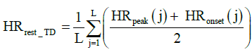
Time domain framework for resting HR estimation: The general framework for resting HR module using time domain method is depicted in Figure 2. The time domain method contains the blocks such as spike removal, smoothing, delineation, outlier’s removal, and HR estimation. The windowed PPG samples are given to the pre-processing stage of the algorithm to remove the sudden spikes from the signal and smoothing is done using moving average filters. The smoothing process is required to get the robust impulsive signal, which can be obtained by subtracting the delayed version of the smoothed PPG signal from the original PPG signal. This is useful to get more visible peaks and onsets easier. The impulsive signal is differentiated in the delineator block which is easier to identify peaks and onsets from the signal. In the HR estimation block, valid peaks and onsets are identified to estimate the peak to peak and onset to onset interval correctly.

In the above Figure 2.1 is Delineator Output a) smoothed impulsive signal b) Differential signal c) onsets and peaks. Finally, the HR output is calculated by averaging the valid peaks and onsets pairs which are given in the below Equation,

            (1)

Where HR_{rest_TD} is the final resting HR in time domain analysis method.

HR _peak - Valid peaks in HR signal.

HR _onset -Valid onsets in HR signal.

L- Total no of samples.

Frequency domain framework for resting HR estimation: The general framework for resting HR module using frequency domain method is depicted in Figure 3. The frequency domain method contains the blocks such as sampling rate reduction module, smoothing filter, normalization, Fourier transforms, and HR estimation.

The first stage of the frequency domain algorithm is sampling rate reduction. Here the down sampler is used to reduce the input signal sampling rate to 10Hz since the useful information present in the PPG signal lies in between the frequency band of 0.5Hz to 4Hz. This sampling rate reduction is mainly performed to achieve a high resolution on HR estimation. The down sampling factor is chosen based on the original sampling frequency (Figure 3.1).

The output signal of the down sampler is smoothed using a ‘lowess’ smoothing filter to remove the noises. The impulsive signal is generated by subtracting the smoothed ‘lowess’ filter output from the original PPG signal. The amplitude of the impulsive signal is normalized using Hilbert transform and the normalized output is in discrete time domain format (Figure 3.2).

In order to convert the time domain signal into a frequency domain signal, a 512-point Fast Fourier Transformation block is used. The most dominant frequency component f_max is computed using Peak detection algorithm. HR can be estimated based on the new sampling frequency ‘F_snew’, ‘f_max’ and FFT points ‘N’ which is given below,

                 (2)

Where HR_{rest_FD} is the final resting HR value in frequency domain analysis method.

f_max = dominant frequency component. F_snew = new sampling frequency.

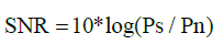
Combined approach of frequency and time domain method: In the combined approach, the Reliability Factor (RF) is calculated based on equation.3 for time domain method and SNR is calculated in equation (4) for frequency domain to estimate HR. Reliability factor can be calculated based on the valid peaks and onsets from the total number of available peaks and onsets, if this factor satisfies the threshold then resting HR value is displayed in the current window otherwise it rejects the current window and moves into the next window datasets. The SNR is calculated by using the signal power (Ps) and the noise power (Pn) from the FFT output signal. Estimated SNR is compared with the SNR threshold value to display the correct HR output. More details about the time and frequency domain can be elaborated in our previous publication [8].

               (3)

              (4)

Tracking Algorithm for Working

Heart Rate Measurement

The block diagram for the tracking framework is shown in Figure 4. Here it uses a raw PPG signal and a simultaneous tri-axial acceleration signal to estimate the HR. As a pre-processing step, the input PPG and accelerometer data are band pass filtered with a cut-off frequency of 0.5 - 4Hz. The filtered PPG is given as primary input and the filtered accelerometer data is given as reference input to the adaptive filter. Hence motion signal present in the primary input is cancelled at the adaptive filter output. The motion arti facts removed adaptive filter output is given as input to the three state-variable filters. The state variable filter filters the signal with varying cut-off frequencies that are obtained using the frequency tracker block. The output of the last state variable filter is fed back to the frequency tracker and the new cut-off frequency is obtained with the help of motion index and the root mean square value of the low pass and high pass filter outputs of the state variable filter. The verification of the calculated frequency is done in the verification module. Finally, the SNR is calculated based on the band pass outputs of the state variable filters and the tracking HR is estimated using the frequency tracker output. The following sections will explain each stage involved in the tracking HR framework.

Pre-processing

The raw input PPG signal and the raw accelerometer data are given to the first stage of the tracking HR algorithm. Here both the signals are band-pass filtered by using infinite impulse response filtering method with a lower cut-off frequency of 0.5 Hz and higher cut-off frequency of 4 Hz with an order of 4, because HR frequency lies in the range of [0.5 - 4] Hz band. After filtering, almost all the environmental noise and motion arti fact outside the frequency band are removed.

Adaptive filtering system

An Adaptive filter is the most popular technique for the removal of motion arti facts with low computational complexity and simpler to design the algorithm. It can adjust its filter coefficients dynamically based on the predetermined initial conditions. The two most popular algorithms are Least Mean Square (LMS) and Recursive Least Square (RLS) and they are utilized to design the adaptive filtering systems. These two algorithms are greatly influenced in arti fact removal and it removes the motion arti fact based on two parameters. The first parameter is the length of the filter and another one is the forgetting factor. Based on the adjustments of these two parameters, arti fact removal can be greatly increased and LMS is potentially simple to implement, but the convergence rate is slow when compared to the RLS filtering method. Therefore, these two methods are analyzed and implemented to provide a more robust solution in our proposed work. Commonly the adaptive systems require reference signals to remove the arti facts where the PPG signal is heavily contaminated with the motion. The general concept behind the system is that the reference input is adaptively filtered and subtracted from the primary signal to get the desired output. In our proposed method, the reference signal is an accelerometer signal which is usually corrupted due to the subject’s movement of hands or during exercise at any instant of time. The primary signal comprising of the desired signal which is arti fact free component is added with the corrupted signal due to the motion. The motion noise is always not correlated with the signal and it varies depending upon the subject's skin colour, sensor positioning, and environmental conditions. The performance of the systems depends on the correlation between the reference signal and motion arti fact components contaminated into the primary signal. In order to compare the performance and to provide a better filtering system model, a two-filtering model namely single-stage and cascaded adaptive systems are designed. Based on the system model usage, a reference signal is created. For single-stage filter, one reference input is used whereas, for cascaded filtering model, instead of employing one reference signal, a tri-axial accelerometer signal used as a reference input to the filter.

Single-Stage Adaptive Filter System Model: Single-stage adaptive filter is a conventional filtering technique to remove the arti facts from the signal. The combined accelerometer signal is considered as a single reference source of input in single-stage adaptive filter instead of using the accelerometer signals separately like cascaded filters (Figure 5). The single-stage adaptive filter is similar to general noise-cancellation techniques and the reference signal is created with the use of three channel accelerometer signals.

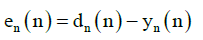
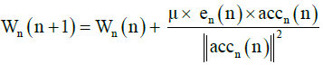
The primary input, reference input and error signals are represented by dn(n), accn(n) and en( n) respectively. wn (n) is a weight update equation based on the order of the filter. The number of filter coefficients are updated instantaneously based on the type of the signal. The working formulas used for designing nth stage LMS filters are expressed as,

               (6)

                 (7)

The Normalized LMS algorithm is the modified form of standard LMS algorithm. In this type, the reference input is normalized, and weight update can be expressed as,

              (8)

is the single stage motion artifact filtered signal.

Algorithm for Recursive Least Square (RLS) filters as follows:

The RLS adaptive filter implementation is as follows

Initialize, the weight vector W and inverse correlation matrix P as

W^H (0) = 0 and P (0) = δ I

Where, δ is the regularization parameter & I is the Identity matrix.

Compute, For each instance of time n = 1, 2, 3 ··· N

                 (9)

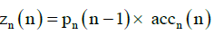
Where w_n(n+1) Is the previous weight vector & acc_n(n) is reference acceleration signal

. i. The error signal is computed by the following equation

                 (10)

Where, e_n (n) is the system output signal & y_n (n) is the adaptive filtered output signal.

            (11)

Where, z_n (n) is the signal used for calculating the Kalman gain vector k_n( n).

               (12)

                     (13)

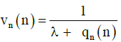
Where q_n (n) & v_n (n) intermediate signals & lambda are in the exponential weighting factor.

ii. The Kalman gain vector k_n(n) can be calculated from intermediate signals are,

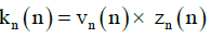               (14)

iii. The weight vector Equation for updating filter coefficients are

                  (15)

iv. The inverse correlation matrix is updated for each iteration which is given by,

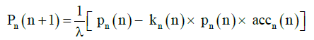               (16)

For reference signal, the three axis captured accelerometer data are squared individually and added together to form a signal, which is used as a reference in single stage filter.

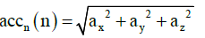              (17)

Where, a_x is the accelerometer data in x-axis, a_y is the accelerometer data in y-axis and a_z is the accelerometer data in z-axis.

Cascaded Adaptive Filter System Model: In this section, three stage cascaded adaptive filter design model is used to remove the arti facts from the corrupted PPG signal. The pre-processed PPG signal along with the accelerometer motion data for three different directions are used for the adaptive filter inputs. In the Figure. 5, the three channel accelerometer data from each channel is used separately as a reference for each adaptive filter

blocks. The reference x-channel input (acc_x ), which is passed into the first stage of the filter blocks. Similarly, acc_yand acc_zare the reference for second and third stage input for y-channel and z-channel respectively. Since these filters are connected in cascaded structure there is a possibility of removing motion artifact higher than compared to single stage filters. From the designed cascaded filter model, it is confirmed that three-stage adaptive filters removed the motion arti facts noise comparatively higher than single stage filtering scheme.

In this case, components of motion artifact present in the PPG signal is removed successively with the reference of x, y, and z directions. Instead of using single stage filter design, the cascaded filter performance is better interms of noise removal from the signal. In the cascaded noise canceller blocks, at the first stage, the input signal to the adaptive filter block is pre-processed PPG signal and reference is the x-channel accelerometer signal represented by mx (n). The output of first stage is used as the input signal of the second one represented by e₁ (n) with the y-channel accelerometer signal m_y (n) being the reference signal. Similarly, for the third stage block the input signal is the output of the second noise canceller represented by e₂ (n) and the reference signal is the z-channel accelerometer signal m_z (n) (Figure 6).

The output represented by y₃ (n) of the final stage is the motion artifact reduced output of the cascaded noise canceller. It is expected that the three stages sequentially remove the motion arti facts corresponding to x, y, and z-channel. The motion arti facts signals presented in the PPG signal represented in terms of a weighted linear combination of three channel accelerometer data, namely m_x (n), m_y (n), m_z (n) in three channel dimensions of movement along x, y and z-axis respectively can be written as in Equation 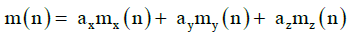(18),

               (18)

Here a_x, a_y, a_z are weighting parameters and their values depend on relative strength of movement in a particular direction. In the single stage and cascaded filtering systems, three different filters LMS, Normalized LMS and RLS were used separately to test the performance of the system model. Hence, these system models have shown the noise performance depending upon the types of filters used in the design. It is observed that RLS filtering has outperformed than other two filters in both the system design and cascaded model has significantly high removal of motion arti facts compared to single stage system model.

State variable filter:

State variable filter adaptively varies the frequency of the signal for peak tracking and verification. The adaptive filtered signal is passed to the state variable filter which gives the low, high, and band pass filter outputs. The digital state variable filter is a popular synthesizer filter. The state variable filter has several advantages over biquad filter. Low pass, high pass and band pass are available simultaneously. In Figure 7, the adaptive filter output is sent as input to the state variable filter. The state variable filter output is fed back to the frequency tracker block to estimate the new cut-off frequency for the variable filter.

Frequency and Q factor are independent and are calculated by the following Equations.

The frequency control coefficient, f, is given by,

                (19)

Where F_s are the sampling rate and F_c is the filters cutoff frequency. The damping factor (q) is given by

                       (20)

Where Q ranges from 0.5 to infinity.

The resulting frequency component is sent to the peak tracking module where the output is given as feedback to the state variable filter to get the required frequency component for determining the HR.

Peak Tracking and Verification:

From the state variable filter the varying frequency output is passed into this module. Peaks in the signal are estimated based on the frequency. The frequencies are tracked, and the cut-off frequency will be varied in real time. Frequency is estimated using the following equation,

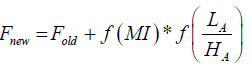              (21)

Where, L_A -Amplitude of Low pass filter output, H_A- Amplitude of High pass filter output, MI - Motion Index

Experimental Results

It is needed to evaluate the estimated HR output to see the effectiveness and the performance of an algorithm at rest and motion conditions. Continuous HR testing is performed for real time validation of the proposed method. In continuous HR testing, the HR output is measured at regular intervals for a limited period of time. For offline validation of HR, the PPG and accelerometer data are collected from different subjects (60 male and 40 female) of different age group (age 21 – 50 years) with different skin tones (dark and fair skin). Also, the participants are asked to give random motions like typing, ball tapping and writing etc. Data collection protocol is given in the following Table 1.

Data Collection:

The dataset for the validation of the algorithm is recorded using a single channel PPG sensor and a tri-axial accelerometer from different subjects with different skin tones of various age groups and they are sampled at 100 Hz. The test cases mentioned in table 1 is considered as a motion arti facts source for our proposed method for heart rate estimation at different scenarios. The factors that are used to identify the performance of the algorithm are as follows,

Pass percentage: The difference between the HR estimated from the proposed method and the reference device are compared with a certain deviation range to decide the accuracy of our proposed HR algorithm. A sample pseudo code is given below.

If (abs (HR_Est - HR_Ref)) < = deviation range

Status = PASS;

else

Status = FAIL;

The deviation region is set to a static value of 5 BPM in our proposed algorithm.

MAPE and MAE: Mean Absolute Percentage Error (MAPE) and Mean Absolute Error (MAE) are the two main deciding factors to evaluate the performance of our proposed algorithm.

The Mean Absolute Percentage Error (MAPE) provides the percentage of accuracy of the algorithm, and it is given by the Equation 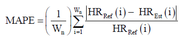(22),

                  (22)

The Mean Absolute Error (MAE) is used to measure the closeness of the estimated HR to the reference HR. It is given by the following Equation (23),

                (23)

Where,

HR_Ref – HR from the reference device, HR_Est – HR from the proposed algorithm, W_n – Total number of windows.

Reference Closeness Factor (RCF): The Reference Closeness Factor is a prominent factor which gives the closeness of the algorithm HR with respect to reference HR in the range from 0 to 1. It is given by the following equation.

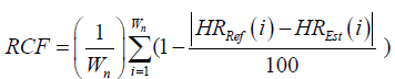                  (24)

Comparison of Test Results

The proposed method is compared to the stand-alone Single Vector Decomposition (SVD) and Independent Component Analysis (ICA) algorithm and the results are given in Table 2. Continuous testing is conducted when the subject is at rest condition and doing mild, medium, and heavy motion. The comparison is made between the proposed method, SVD and ICA method. The proposed method achieves a pass percentage of 98.6% in continuous testing.

The tracking algorithm for estimating HR gives much better performance with a reduced error rate i.e. MAE of 1.18 BPM and MAPE of 1.67% in On-demand testing and it is even very low in continuous testing compared to the standalone methods, which can also be seen in the Table 2.

The proposed method gives the first heart rate output at 6.06 seconds average which is faster than other algorithms. In continuous testing, the response time is not applicable because HR monitoring is a continuous process.

The proposed method is implemented in C and ported to the cortex M4 platform for validation, since wearable devices are using ARM processors mostly. The main reason for proposing this method is for the accuracy of heart rate output compared to the other available methods, which is the primary factor in measuring the heart rate in real time applications. The hardware resources required for the proposed model is given below in the following Table 3.

Real Time Applications

The proposed framework is initially implemented and validated in MATLAB using offline PPG data. The estimated output is compared with the reference HR available in the database and based on the pass percentage, the algorithm is fine-tuned. Once the performance of the algorithm is validated fully, then the real time implementation is preceded. For real time implementation, the MATLAB algorithm is converted into C code and it is built for ARM cortex M4 processor using IAR embedded workbench. The resultant binary is flashed into the M4 evaluation board. A sample android application is developed to display the HR results estimated from the M4 board. The application and Cortex M4 board are communicated through Bluetooth to display the HR in android application GUI (Figure 8).

Conclusion

A general framework for calculating the HR at all possible conditions is proposed in this paper. Since HR is a vital parameter in health care devices, this proposed framework can be used to calculate HR when the subject is at rest or regular activities based on the combination of time domain, frequency domain, and tracking using accelerometer data. From the experiments conducted, it is proved that the proposed framework is giving better results when compared with the HR estimated from the other methods. The accuracy of the proposed framework in real time environment is 98.6 % achieved and the MAPE is 1.67 %, MAE is 1.18 BPM and the RCF is 0.987. The hardware implementation of the algorithm requires total of 47KB memory which runs at a speed of 5.7 MIPS.

References

1. Islam Md Saiful, and Naif Alajlan. "Augmented-hilbert transform for detecting peaks of a finger-ECG signal." In 2014 IEEE Conference on Biomedical Engineering and Sciences (IECBES), IEEE (2014) 864-867.
2. Andrienko, Gennady, Natalia Andrienko, Martin Mladenov, and Michael Mock, et al. "Extracting events from spatial time series." In 2010 14th International Conference Information Visualisation, IEEE (2010) 48-53
3. Zong W, Heldt T, Moody G B, and Mark R G. "An open-source algorithm to detect onset of arterial blood pressure pulses." Comput Cardiol IEEE (2003): 259-262.
4. Elgendi Mohamed, Mirjam Jonkman, and Friso De Boer. "Measurement of aa intervals at rest in the second derivative plethysmogram." Proceedings of the IEEE (2009): 75-79.
5. Elgendi Mohamed, Ian Norton, Matt Brearley, andDerek Abbott, et al. "Systolic peak detection in acceleration photoplethysmograms measured from emergency responders in tropical conditions." PLoS One 8 (2013): 1- 11.
6. Elgendi Mohamed, Ian Norton, Matt Brearley, and Derek Abbott, et al. "Detection of a and b waves in the acceleration photoplethysmogram." Biomed Eng Online 13 (2014): 1-18.
7. Elgendi, Mohamed, Mirjam Jonkman, and Friso DeBoer. "Heart rate variability and the acceleration plethysmogram signals measured at rest." In International Joint Conference on Biomedical Engineering Systems and Technologies 127 (2010): 266-277.
8. Ram M Raghu, K Venu Madhav, E Hari Krishna, and Nagarjuna Reddy Komalla, et al. "A novel approach for motion artifact reduction in PPG signals based on AS-LMS adaptive filter." IEEE Trans Instrum Meas 61 (2011): 1445-1457.
9. Lee Han-Wook, Ju-Won Lee, Won-Geun Jung, and Gun-Ki Lee. "The periodic moving average filter for removing motion artifacts from PPG signals." Int J Control Autom Syst 5 (2007): 701-706.
10. Ram M Raghu, K Venu Madhav, Ette Hari Krishna, and Nagarjuna Reddy Komalla, et al. "ICA-based improved DTCWT technique for MA reduction in PPG signals with restored respiratory information." IEEE Trans Instrum Meas 62 (2013): 2639-2651.
11. Kim Byung S, and Sun K Yoo. "Motion artifact reduction in photoplethysmography using independent component analysis." IEEE Trans Biomed Eng 53 (2006): 566-568.
12. Reddy K Ashoka, and V Jagadeesh Kumar. "Motion artifact reduction in photoplethysmographic signals using singular value decomposition." In 2007 IEEE Instrumentation & Measurement Technology Conference IMTC 2007, IEEE (2007): 1-4.
13. Raghuram M, K Venu Madhav, E Hari Krishna, and K Ashoka Reddy. "Evaluation of wavelets for reduction of motion artifacts in photoplethysmographic signals." In 10th International Conference on Information Science, Signal Processing and their Applications IEEE (2010): 460-463.
14. Gilles Jerome. "Empirical wavelet transform." IEEE Trans Signal Process 61 (2013): 3999-4010.
15. Sun Xuxue, Ping Yang, Yulin Li, and Zhifan Gao, et al. "Robust heart beat detection from photoplethysmography interlaced with motion artifacts based on empirical mode decomposition." In Proceedings of 2012 IEEE-EMBS International Conference on Biomedical and Health Informatics, IEEE (2012): 775-778.
16. Nowak Ewelina, Mateusz Kraiński, Maciej Rubiński, and Marta Pazderska, et al. "Robust real-time PPG-based heart rate monitoring." In 2015 23rd European Signal Processing Conference (EUSIPCO), IEEE (2015): 2561-2565.
17. Zhang Zhilin, Zhouyue Pi, and Benyuan Liu. "TROIKA: A general framework for heart rate monitoring using wrist-type photoplethysmographic signals during intensive physical exercise." IEEE Trans Biomed Eng 62 (2014): 522-531.
18. Zhang Zhilin. "Photoplethysmography-based heart rate monitoring in physical activities via joint sparse spectrum reconstruction." IEEE Trans Biomed Eng 62 (2015): 1902-1910.
19. Sun Biao, and Zhilin Zhang. "Photoplethysmography-based heart rate monitoring using asymmetric least squares spectrum subtraction and bayesian decision theory." IEEE Sens J 15 (2015): 7161-7168.
20. Zhang Yangsong, Benyuan Liu, and Zhilin Zhang. "Combining ensemble empirical mode decomposition with spectrum subtraction technique for heart rate monitoring using wrist-type photoplethysmography." Biomed Signal Process Control 21 (2015): 119-125.
21. Yousefi Rasoul, and Mehrdad Nourani. "Separating arterial and venous-related components of photoplethysmographic signals for accurate extraction of oxygen saturation and respiratory rate." IEEE J Biomed Health Inform 19 (2014): 848-857.
22. Yousefi Rasoul, Mehrdad Nourani, Sarah Ostadabbas, and Issa Panahi. "A motion-tolerant adaptive algorithm for wearable photoplethysmographic biosensors." IEEE J Biomed Health Inform 18 (2013): 670-681.
23. Mohan P Madhan, V Nagarajan, and J C Vignesh. "Spot and continuous monitoring of heart rate by combining time and frequency domain analysis of photoplethysmographic signals at rest conditions." IET Signal Processing 11 (2017):1076-1082.