Analyzing the Contribution of Indian Civil Industry to Economic Growth in the Pre-covid Era: An ARDL Approach

Priyanka Saharia^*
*Correspondence: Priyanka Saharia, Department of Public Policy, Manipal Academy of Higher Education, Bengaluru, India, Email: ,

Keywords

Civil aviation • Economic growth • ARDL • IAA

Classifications

Economics

Introduction

The present study deals with the contribution of the civil aviation industry to economic growth. As is known, the transport sector and related infrastructure have played a pivotal role in the economic development of a region and the economy. The transport sector and its role in economic growth are well documented in both theoretical and empirical literature. In recent years, air transportation has become the fastest-growing mode of transportation in India. The rapid economic growth and a growing middle-class population have brought tremendous demand for air transportation. According to the DGCA, domestic passengers’ traffic expanded at a CAGR of 13.52 per cent from FY2006 to FY2017 while the international passengers' traffic increased by 8.5 percent for the same period. Total freight registered a CAGR of 7.08 per cent from FY2006 to 2017. The cargo and passengers’ growth of the industry has significant impact on expansion of airport infrastructure and growth of the Indian civil aviation industry. The civil aviation industry is known to have its direct, indirect, and induced impact on economic growth. The direct impact includes the activities in the air transport industry, indirect economic impact implies the employment and economic activities in the air transport industry's supply chain, and induced impacts express employment and economic activities supported by the spending of those employed in the direct and indirect sectors [1].

With the growing demand for air travel, the industry's contribution to economic growth also requires attention from researchers. Therefore, to understand the growing importance of civil aviation, as a mode of transportation and its role in the national economy, this study aims to investigate the direct contribution of the civil aviation industry to economic growth. Further, it adds various macroeconomic variables to strengthen the analysis. The present chapter also attempts to analyze the causal relationship between economic growth and the civil aviation industry. To begin with, in the below section, the relationship between growth of air passengers’ traffic and GDP in India is explained.

Relationship between air passengers traffic and GDP in India

The present section analyzes the relationship between the growth rate of air passengers’ traffic and GDP in India. The total numbers of passengers carried by air travel are considered for passengers' growth and GDP at factor cost is considered to represent the economic growth. The period of the analysis is from 1981 to 2018. The trend of GDP and air passengers’ growth is presented in Figure 1.

Figure 1 illustrates a positive relationship between air passengers’ growth and GDP. The CAGRs of passengers carried and GDP are estimated to understand the pattern of their growth. It is observed from Figure 1 that passenger’s growth rates have always been more than the growth rates of GDP. The CAGRs of passengers’ growth can be divided into two phases; from 1981 to 2000 can be considered as the low growth phase and from 2001 to 2018 can be considered as the high growth phase. In the low growth phase, the CAGRs of passengers carried are moderately higher than the CAGRs of GDP, while in the high growth phase, CAGRs of passengers carried are double the CAGRs of GDP. The higher air traffic growth rate in the post- 2000 can be attributed to the entry of low-cost airlines in the Indian domestic aviation market. After the deregulation of the industry, low-cost carriers started operating in the Indian aviation market and it led to the growth of air passengers’ traffic. The low-cost airlines made air travel accessible to common people by charging low airfares [2]. The growing middle-class population and rise of per capita income are also important factors that contributed towards the passengers' growth of the industry. Further, it can be also observed that from 2001 to 2018, the relationship between the growth rate of passengers traffic and GDP is approaching the often-cited rule of thumb throughout the airline industry which states that "demand for air travel grows twice as fast as gross domestic product".

The present study also looks at the growth rate of the air transport component of the civil aviation industry in terms of its output over time. For this, the annual growth rate of the output is estimated from 1981 to 2019 and it is presented in The present study also looks at the growth rate of the air transport component of the civil aviation industry in terms of its output over time. For this, the annual growth rate of the output is estimated from 1981 to 2019 and it is presented in Figure 2.

Figure 2 illustrates that the growth rate of output is declining continuously from 1982 and it is becoming negative from 1990 to 1993. The reason for the negative growth rate of output can be attributed to the period of economic reform when GoI brought changes in civil aviation policy. In 1994, the Government decided to repeal of Air Corporation Act, 1994 and started deregulating the Indian civil aviation industry. It ended the monopoly nature of the Indian airline industry and allowed private airlines to operate in the market [3].

The drops in aviation output growth rate from 2000 to 2002 can be attributed to the combined 2000-2001 shock of the dot-com bust and the world trade center attack of 9th September 2011. From 2002-07, the movement of aviation output starts increasing continuously and reaches its peak in the year 2006. The entry of low-cost carriers in the post-2002 is the major reason for the boom of the industry as it increased the demand for air travel due to the lower ticket fare, making air travel accessible to a wider section of the population than earlier. The growth rate of civil aviation output drops again in 2008-09 followed by the global financial crisis. The world aviation industry was severely affected by the impact of the global financial crisis and the Indian aviation market was also not an exception [4]. Further, the output growth rate drops during 2012-13, due to the grounding of kingfisher and the global economic scenario. The other important causes include high airport charges and maintenance costs, higher operating costs, high and growing debt burden and huge taxation on aviation turbine fuel of the industry. The economic times reports that according to the Government of India, the civil aviation industry has a total loss of Rs 5,389 crore in 2012-13.

Figure 2 shows the growth rate of output of the civil aviation industry is very volatile and therefore it can be concluded that the growth of the civil aviation industry is subject to the various global and regional economic as well as political factors.

Methodology

Data sources

The sources of data and variables used for the present study are mentioned in this section. The contribution of the civil aviation industry to economic growth is analyzed using the variables namely, GDP at factor cost, the output of air transportation industry, WPI of ATF, Real Effective Exchange Rate (REER), and total export of the country. To avoid the problem of double counting, the output values of the air transportation industry are deducted from GDP at factor cost. The period of the study is from 1981 to 2019 with the annual time series data. Data on selected variables are collected at constant price and converted to one common base year price i.e, 2011-12. The study also has checked for structural breaks and found that there are two structural breaks in the model to be estimated; one is in 1994 and another one is in 2008. The structural break in 1994 can be attributed to the policy changes due to economic reforms in India. The Indian civil aviation industry was also deregulated in the year 1994 as a result of economic reforms. The reason for the structural break in 2008 can be considered due to the global financial crisis as economic activity declined in half of all the countries in the world. As a result of the financial crisis, the global aviation industry was one of the worst-hit industries and the Indian aviation industry was not an exception [5]. Hence two dummy variables are included, namely d1 and d2. From the year 1981 to 1993 is considered as 0 and from 1994 to 2019 is considered as 1 to represent d1. To represent d2, from 1981 to 2008 is considered as 0 and from 2008 to 2019 is considered as 1. The variables and data sources are presented in Table 1.

The GDP at factor cost is considered as the dependent variable to represent economic growth in the study. The study focuses on the direct contribution of the civil aviation industry to economic growth. In line with The 'Report of Working Group on Civil Aviation Sector' by MoCA, the present study considers the air transport component of the civil aviation industry to represent its contribution to economic growth. Therefore, the total output value of the Indian air transportation industry is taken as the key explanatory variable for the econometric estimation to represent the contribution of the civil aviation industry to GDP [6].

Total export of the country is another explanatory variable for the study. Export plays an important on the economy in the economic growth of a country. Air transportation also has a significant impact on export as air freight represents 35 per cent of global trade value though it contributes less than 1 per cent of global trade volume. WPI of ATF is considered as another independent variable for the estimation. WPI of ATF represents the price of ATF and how it impacts the economy. In the world of globalization, the exchange rate plays a major role in every country's economic activity. The trade-based REER is considered to represent the exchange rate [7,8].

In Table 2, descriptive statistics of all the selected variables are presented.

The Descriptive statistics of the variables are provided before the econometric estimation. To check whether the data series is normally distributed, the Jarque-Bera test statistic is carried out. The proposed hypothesis for the Jarque-Bera test is

H₀: Data is normally distributed and

H_a: Data is not normally distributed

The null hypothesis will be accepted when the p-value is greater than 0.05 and rejected otherwise. From Table 2, p-values of GDP, export, and WPI of ATF are greater than 0.05. Therefore, the null hypothesis is accepted stating that data is normally distributed. For output and REER, the p-value is smaller than 0.05 and hence the null hypothesis is rejected. However, generally, time-series data tend to show a growing trend due to the time factor and it can be seen in Figure 3 representing the raw data of the current study [9].

Figure 3 suggests the existence of trends in all variables. The variables are then tested for stationarity to verify the existence of trends and to understand the order of integrations in section 3.2. To reduce the variation in the variables, all the variables are transformed to their natural logarithmic form for the estimation.

Result of unit root test

The unit root test enables us in understanding the characteristics of data and selecting a suitable model for the analysis. Table 3 represents the unit root test result for all the variables. There are several tests to carry out the unit root test. Phillip-Perron, Augmented Dicky Fuller (ADF) and KPSS are most commonly used test to check the order of integration of each variable. In the present study, the Augmented Dicky Fuller (ADF) is used to check for the stationarity of the variables. The result of the ADF test helps in deciding upon the model for further analysis. As per the result of the unit root test, all the variables are non-stationary and integrated to the first order. In such a scenario, for econometric analysis, a study can adopt either the Vector Error Correction Model (VECM) or the Autoregressive Distributed Lagged model (ARDL). However, ARDL has advantages over VECM in the case of a small sample size. The advantages of the ARDL model are explained in the below the ARDL model section [10].

The ARDL model

In this section, the rationale behind the econometric model used to estimate the short-run and long-run relationship between economic growth and the civil aviation industry is explained. GDP at factor cost is considered as the dependent variable. Key independent variables of the model are the output of the air transport industry, export, WPI of ATF, and REER. The study has adopted an ARDL model over the VECM for the numerous advantages such as ARDL model distinguishes the dependent and independent variables whereas, in the VECM, all the variables are endogenous. ARDL also allows the variables of estimation to have different optimal lags. It employs a single reduced from equation [11] and it estimates both long-run and short-run components of the model simultaneously, removing problems associated with omitted variables and autocorrelations [12]. The structural break for the model is also checked and found that there is a structural break in the years 1994 and 2008, and these breaks are considered as dummy variables in the model. Based on the variable description, the proposed model of estimation is defined below:

In(GDPt) = β0 + β1 In(OUTPUTt) + β2In(EXPORTt) + β3In(WPIt) +β4InREER + γ1D1t + γ2D2t+ Ut ………… (1)

In the above equation, InGDP represents the economic growth of the country, the output represents the total value of air transport component to represent the civil aviation industry, export represents overall export of the country, WPI represents the wholesale price index of ATF and REER is the real effective exchange rate. D1t and D2t represent the dummy variables here. All the variables have been taken at a constant price of 2011-12.

For causal analysis, the Innovative Accounting Approach (IAA) is used. IAA is used to measure the causal relationship among the variables. The advantage of IAA over the Granger Causality test is that it explains how much extent of feedback exists from one variable to the other. The Granger causality test shows the causal relationship among the variables within the sample period. IAA illustrates the causal relationship ahead of the selected sample period. Another significant advantage of IAA, it is not sensitive to the order of integration of variables in the VAR. Pesaran and Shin pointed out a proportional contribution in one variable due to an innovative shock caused by another variable is shown by the generalized forecast error variance decomposition method. Hence, the present study used IAA to understand the causal relationship between economic growth and civil aviation growth. IAA applies impulse response function to determine the causal relationship ahead of the sample period. An impulse response function traces the effect of one standard deviation shock to one of the innovations on the current and future values of the endogenous variables. In the present study, impulse response function over a range of 10 year periods is shown through the VECM dynamic structure.

The econometric model

ARDL approach is a co-integration technique for determining the long-run and short-run relationship among the variables of the study. Considering the advantages of the ARDL approach over the vector error correction approach mentioned in section The ARDL model, the following equation is specified. For the short-run dynamic, the equation is as follows:

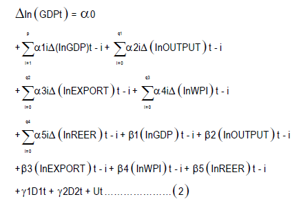
In the equation (2), Δ is the first difference operator, q is the optimal lag length, α1i, α2i, α3i, α4i and α5i represent the short-run dynamics of the model, and β1, β2, β3, β4, and β5 represent the long-run dynamics of the model.

Selection of optimal lags length: For a correct model specification, before the estimation, it must to specify the length of the lags. All inferences in the model depend on the correct model specification. We choose the lag length of the VAR in levels that minimizes the information criteria. The lag length of the model is selected through the Akaike Information Criterion (AIC), Schwarz Criterion (SC), and Henna-Quinn (HQ). But most commonly used information criterion for selecting optimal lags length are the AIC and SC. This study would adopt the AIC. Table 4 represents the optimal lag length for the present study which is 2 according to the AIC.

An error correction version of equation (2) is

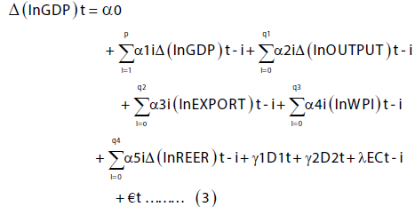
In the equation (3), λECt-I represents the error correction term that tells about the speed of adjustment towards the long run equilibrium.

Bound test for long-run relationship: To find out if a long-run relationship exists between the variables, as it is given in equation (1), a Bound test for equation (2) is conducted. The bound test considers two bounds: upper bound and lower bound. The null hypothesis for the test assumes that there is no cointegration among the variables in the long run. The rule of thumb for the Bound test approach is, if the calculated value of F-statistics is more than the upper bound value then there is cointegration among the variables and it rejects the null hypothesis. If the value of F-statistics is less than the lower bound, then the null hypothesis is accepted implying that there is no long-run relationship between the variables. The Bound test for cointegration is run on the long-run coefficient of the variables.

Hypothesis set for the Bound test

H₀: β1=β2=β3=β4=β5=0

H_A: β1 ≠β2 ≠β3 ≠β4 ≠β5≠ 0

Table 5 presents the result of the bound test. The upper bound is indicated by I (1) and lower bound is indicated by I (0).

The result of the bound test in Table 5 shows that the calculated value of F-statistics is more than the value of the upper bound i.e., I (1). Therefore, the null hypothesis is rejected and concluded that there is a long-run relationship between the variables. The existence of co-integration among the variables allows us to estimate the ARDL model.

Results and Discussion

Table 6 represents the error correction results of the selected ARDL (2, 2, 0, 1, 0) model. Coefficients with variables D-sign shows the short-run elasticity. Error correction term tells us about the speed of adjustments towards the longrun equilibrium. If the dependent variable has moved away from equilibrium in the short run, the error correction term captures how long it will take for the dependent variable to come back to equilibrium compare to the previous year's disequilibrium.

The present study included d1 and d2 in the model to represent the structural breaks in 1994 and 2008 respectively. D1 is negatively related to economic growth, and it is significant at the 10 percent level implying that the economic reform period is negatively related to economic growth. The Indian civil aviation industry was also deregulated in the year 1994 and major policy changes took place across the various segments of the economy. The d2 is also significant and negatively impacts economic growth in the study implying that due to the global financial crisis of 2008, economic growth has declined in the short run. The other two explanatory variables, WPI of ATF and EXPORT are also significant at their first lag. The WPI of ATF is negatively related to economic growth and EXPORT is positively related to economic growth.

The value of the error correction term indicates that the speed of adjustment process from the previous year's disequilibrium in the economic growth to the current year is around 36 per cent and it is highly significant with a p-value of 0.0000. The result of the long-run estimation is presented in Table 7.

The co-efficient value output in the long-run estimated equation indicates that the output of the industry is positively related to economic growth implying a one percent increase in output is associated with an increase in economic growth by 0.28 percent. Output is significant at a 5 per cent level of significance. This finding is in line with the findings of Hakim MM and Merkert R [13], Marazzo M, et al. [14] and Mehmood B, et al. [15] who found a positive relationship between aviation demand and economic growth.

Export is also positively related to economic growth. The estimated result shows a one percent increase in export leads to an increase in economic growth by 0.43 percent approximately. This empirical result is supported by Guntukula R [16] and Ray S [17] who find that there is a positive impact of exports on economic growth. Agrawal P [18] found that following the economic reform, the growth of export has played a substantial role in increasing the growth rate of India.

WPI of ATF is negatively related to economic growth. Other things remaining constant, a one percent increase in WPI of ATF is associated with a decrease in economic growth by 0.28 percent. The negative relationship between inflation and economic growth is supported by Barro RJ [19], who finds that a 10 percent increase in inflation per year reduces the GDP-per capita by 0.2-0.3 percent. Berument H, et al. [20] find a negative relationship between inflation and growth.

Result of the diagnostic test

Stability of the model: The stability of the selected ARDL model is tested based on the error correction model using the Cumulative Sum of recursive residuals (CUSUM) and Cumulative Sum of Squares of recursive residuals stability (CUSUMSQ) testing technique. The CUSUMQ and CUSUMSQ plots have been shown in Figure 4 and Figure 5.

The purpose of CUSUM and CUSUMSQ is to check the structural stability of the model. The rule of thumb is if both the plots remain within the critical bounds at a 5 per cent level of significance, it can be concluded that the model is structurally stable. Figure 4 and Figure 5 show that for both CUSUM and CUSUMSQ tests, the plot remains within the critical bounds. Thereby, stating that the estimated ARDL model with the bound test approach is structurally stable. The CUSUM test has higher power if the break is in the intercept of the regression equation. However, if the structural change is in the slope coefficient or the variance of the error term then the CUSUMSQ test has more power.

Result of serial correlation and heteroscedasticity: It is important to check the presence of serial correlation and heteroscedasticity of the model. The problem of serial correlation occurs when the error terms in the regression equations are correlated. The serial correlation will not affect the unbiasedness and consistency of the OLS estimator, but it affects their efficiency. With a positive serial correlation, the standard errors of the OLS estimates will be smaller than the true standards error. In the presence of serial correlation, we conclude that parameter estimates are either less precise or more precise than they are. To avoid this problem, a null hypothesis is formulated with the assumption of no serial correlation in the error term [21].

The presence of heteroskedasticity affects the estimation and test of the hypothesis. To avoid this problem, we test the Breusch-Godfrey test for heteroscedasticity. The null hypothesis set for the test assumes there is no heteroscedasticity. Table 8 shows the result of Breusch- Godfrey test for serial correlation and the Breusch-Godfrey test for heteroscedasticity. The result of the Breusch- Godfrey serial correlation shows that the estimated probability value is 0.66. Since the probability value is greater than 0.05, the null hypothesis is accepted stating that the estimated ARDL model is free from serial correlation.

The result of the Breusch-Godfrey heteroscedasticity shows that the estimated probability value is 0.43 and it is greater than 0.05. Therefore, null hypothesis is accepted and concludes that the estimated ARDL model is free from the presence of heteroscedasticity.

Result of IAA for causality analysis: The direction of causality between economic growth and output of civil aviation is analyzed using the IAA. The IAA combines variance decomposition analysis and impulse response function to determine the causality ahead of the sample function. In this chapter, we present the result of the impulse response function. The period of the present analysis is from 1981 to 2019. Figure 6 shows the causality ahead of 10 years of the sample function.

The impulse response function in Figure 6 illustrates the response of a dependent variable due to forecast error stemming shocks in the independent variables in the model. The impulse response function shows that there is a positive response in economic growth due to a standard shock stemming from the output of the civil aviation industry. It implies economic growth rises, reaches to peak, and starts falling with the continuous output growth of the civil aviation industry. Economic growth reaches its maximum after 4 years. However, the response of civil aviation output due to an innovative shock in economic growth witnesses a continuous increase in it. Economic growth is reacting quickly and significantly to an innovative shock in the output of civil aviation but the output of civil aviation impacted by a shock in economic growth increased suddenly and the more moderated way in the long run.

Conclusion

The study investigates the direct contribution of the civil aviation industry to economic growth for the period 1981 to 2019. To establish a dynamic relationship between the selected variables, the ARDL model is used. The bound test approach is used to deal with the existence of co-integration between the variables in the long run where the error correction method is used to find the short-run dynamics. Further, the IAA approach is used to analyze the direction of causality between economic growth and the civil aviation industry.

In the study, the CAGRs of passengers’ traffic and economic growth shows passengers' growth is higher than economic growth. In post-2000, passengers' growth rate is increasing at double the rate of economic growth, reiterating that demand for air travel grows twice as fast as GDP. The passengers' growth rate at double the rate of GDP makes the entry of low-cost carriers a significant event for the industry. The growth rate air transportation industry is also calculated to represent the growth of the civil aviation industry in the present study and it is found that growth rates of the civil aviation industry, in general, are seen to be highly susceptible to various economic and political factors such as fall of the world trade center, economic slowdown and changes in policy measures, etc.

The empirical finding of the study shows that the output of the civil aviation industry is positively related to economic growth. The co-efficient value of the output shows, economic growth increases by 0.28 per cent when the output of civil aviation increases by 1 per cent during the study period. In the present study, the contribution of the civil aviation industry to economic growth is considered in terms of the output value of the air transport component of the industry. Noninclusion of indirect and induced contribution has reduced the co-efficient value of civil aviation output to economic growth since the most important contribution aviation makes to the economy is through its catalytic impact. Further, despite the aviation boom, the Indian civil aviation industry is heavily dependent on aircraft built by foreign aircraft makers such as Boeing, Airbus, and ATR. The meager direct contribution of the booming aviation industry to economic growth indicates that apart from air passengers' traffic and airport services, the Indian civil aviation industry needs to focus on manufacturing commercial aircraft within the country and strengthen the aircraft manufacturing segment. The focus shall be also given to strengthen the Maintenance, Repair and Overhaul (MRO) sectors of the industry by attracting more investment and increasing the potential to promote employment generating activities in the economy.

To measure the causal analysis, an IAA is used. The causal relationship is explained only among the variables of interest. i.e between economic growth and civil aviation output. The result of the impulse response function shows that there is bi-directional causality between economic growth and the civil aviation industry. Economic growth reacts quickly and significantly to one standard deviation shock in the output of the civil aviation industry however, a shock in economic growth has a meaningful impact on civil aviation output at the end of the observed ten periods as it continues to increase. Hence, the response of civil aviation output to a shock in economic growth is much stronger in the long run and the response of economic growth to civil aviation growth is much stronger and quicker in the short run. The direction of causality indicates the growth of the civil aviation industry will boost the economy in the short term and a boost in overall economic activity will increase the aviation output in long run.

The finding of the present study helps lime lighting the contribution of the Indian civil aviation industry to economic growth. Further, it also draws some policy implications by suggesting focusing on aircraft manufacturing and MRO segments of the industry to increase its direct contribution to economic growth.

Acknowledgement

None.

Conflict of Interest

None.

References

1. Mehmood, Bilal, Acleo Feliceo and Amna Shahid. "What causes what? Aviation demand and economic growth in Romania: Cointegration estimation and causality analysis." Rom Econ Bus Rev 9 (2014): 21-34.

   Google Scholar

2. Mehmood, Bilal and Amna Shahid. "Aviation demand and economic growth in the czech republic: Cointegration estimation and causality analysis." Statistika: Stat & Econ J 94 (2014).

   Google Scholar

3. Baker, Douglas, Rico Merkert and Md Kamruzzaman. "Regional aviation and economic growth: Cointegration and causality analysis in Australia." J Transp Geogr 43 (2015): 140-150.

   Google Scholar, Crossref, Indexed at

4. Van De Vijver, Elien, Ben Derudder and Frank Witlox. "Exploring causality in trade and air passenger travel relationships: The case of Asia-Pacific, 1980–2010." J Transp Geogr 34 (2014): 142-150.

   Google Scholar, Crossref, Indexed at

5. Fernandes, Elton and Ricardo Rodrigues Pacheco. "The causal relationship between GDP and domestic air passenger traffic in Brazil." Transp Plan Technol 33 (2010): 569-581.

   Google Scholar, Crossref, Indexed at

6. Button, Kenneth and Junyang Yuan. "Airfreight transport and economic development: An examination of causality." Urban Studies 50 (2013): 329-340.

   Google Scholar, Crossref, Indexed at

7. Mukkala, Kirsi and Hannu Tervo. "Regional airports and regional growth in Europe: Which way does the causality run." Environ Plan A 45 (2013): 1508-1520.

   Google Scholar

8. Cecilmis, Nisa and Aylin Kos. "Economic factors affecting aviation demand: Practice of EU countries." Curr Prob Econ 5 (20): 412-420.

   Google Scholar, Indexed at

9. Hu, Yi, Jin Xiao, Ying Deng and Yi Xiao, et al. "Domestic air passenger traffic and economic growth in China: Evidence from heterogeneous panel models." J Air Transp Manag 42 (2015): 95-100.

   Google Scholar, Crossref, Indexed at

10. Chang, Yu-Hern and Yu-Wei Chang. "Air cargo expansion and economic growth: Finding the empirical link." J Air Transp Manag 15 (2009): 264-265.

    Google Scholar, Crossref, Indexed at

11. Ozturk, Ilhan and Ali Acaravci. "CO2 emissions, energy consumption and economic growth in Turkey." Renewable Sustainable Energy Rev 14 (2010): 3220-3225.

    Google Scholar, Crossref, Indexed at

12. Narayan, Paresh Kumar. "Fiji's tourism demand: The ARDL approach to cointegration." Tour Econ 10 (2004): 193-206.

    Google Scholar, Crossref, Indexed at

13. Hakim, Md Mahbubul and Rico Merkert. "The causal relationship between air transport and economic growth: Empirical evidence from South Asia." J Transp Geogr 56 (2016): 120-127.

    Google Scholar

14. Marazzo, Marcial, Rafael Scherre and Elton Fernandes. "Air transport demand and economic growth in Brazil: A time series analysis." Transp Res E Logist Transp Rev 46 (2010): 261-269.

    Google Scholar, Crossref, Indexed at

15. Mehmood, Bilal, Amna Shahid and Zahid Irshad Younas. "Interdepencies between aviation demand and economic growth in India: Cointegration equation estimation." Economic Affairs 58 (2013): 337-347.
16. Guntukula, Raju. "Exports, imports and economic growth in India: Evidence from cointegration and causality analysis." Theor & Appl Econ 25 (2018).

    Google Scholar, Indexed at

17. Ray, Sarbapriya. "A causality analysis on the empirical nexus between export and economic growth: Evidence from India." nexus 1 (2011).

    Google Scholar, Indexed at

18. Agrawal, Pradeep. "The role of exports in India's economic growth." J Int Trade Econ Dev 24 (2015): 835-859.

    Google Scholar, Crossref, Indexed at

19. Barro, Robert J. "Education and economic growth." Ann Econ Financ 14 (2013): 301-328.

    Google Scholar, Indexed at

20. Berument, Hakan, Ali Inamlik and Hasan Olgun. "Inflation and growth: Positive or negative relationship?." J Appl Sci 8 (2008): 192-204.

    Google Scholar, Crossref, Indexed at

21. Hui-yun, Zhang and Zhu Mei-gui. "An empirical research on the relation between the air transportation and economic growth." In 2011 International Conference on Management Science & Engineering 18th Annual Conference Proceedings, IEEE (2011): 662-667.

    Google Scholar, Crossref, Indexed at

22. “Review of the classification and definitions used for civil aviation activities.” Montreal: International Civil Aviation Organization. (2009).
23. “The future is bright but not without its challenges.” Geneva: International Air Transport Association. (2019).