Computational Investigation of Complexity and Robustness in Neural Circuits

Jeffrey E. Arle^1,2,3* and Longzhi Mei^1,2
*Correspondence: Jeffrey E. Arle, Department of Neurosurgery, Beth Israel Deaconess Medical Center, 101 Tech Valley Dr., Westford, MA 01886, USA, Email:

Keywords

Complexity • Non-linear • Dynamical systems • Connectome • Neural circuit • Stability • Robustness • Resilience • Systems biology • Functional connectivity

Introduction

To survive and reproduce, biological systems have evolved high levels of resilience to perturbation, also referred to as ‘robustness’ the ability to maintain functionality within astronomically large parameter spaces [1,2]. Bernard C, [3] best known for deep philosophical observations on the proper conduct of biological science and inventing ‘blind’ experimental methods, also played a significant role in developing the concept of homeostasis in biological systems, later refined by Cannon WB [4]. Bernard and Cannon identified homeostasis with the living system’s tendency to maintain a ‘healthy state’ despite continuous inputs from within and without to perturb the healthy state, and if perturbed beyond a limit, to enter a diseased state. Stability and its relationship to complexity has been studied in biological systems at many levels from ecology to cellular biomolecules [5-8].

At some meta-level, such as the ‘operating system’ of the brain and spinal cord, analogous to the operating system of complex software hierarchies, neural circuits’ overall functions are stably maintained despite extensive cell and circuit ‘reformatting’ (property modulation) throughout infant, child and adult life and despite enormous variation in the dynamic range of external input. Moreover, though properties at any systems level in the nervous system may be altered due to disease or degeneracy during normal aging [9-13], even with large amounts of neural component loss or disruption, up to a certain point, general stable function is maintained. For instance, animal models predict that 80% of the dopaminergic neurons in the substantia nigra must be lost for movement disorder symptoms to appear in Parkinson’s disease [14].

One evolutionary strategy for network robustness is redundancy, as seen in von Neumann’s biologically-inspired ‘multiple line trick’ to endow automata with unlimited robustness or as is engineered into the internet’s ability to transmit a message from node A to node B under connectivity loss [15-20]. When a circuit fails with damage, circuit redundancy may permit continuation or restoration of function. Redundant circuit copies may differ from each other, which may offer the system more chance to adapt to environmental challenges. In this sense, the more complexity built into the system, the more robust its potential integrity. Modularity is a second evolutionary strategy to stabilize connectomes. It is present in conserved features across species, from C. elegans to humans, and in more complex organisms, a concentrated central network hub and smallworld topology that evolved for different reasons [2]. Hierarchical organization may be a third evolutionary strategy [21].

However, redundancy, modularity, and hierarchical organization may not be the only evolutionary strategies for robustness and may not be sufficient in all network structure classes. For instance, if each component is simple, non-complex, and not highly interconnected, when circumstances defeat one element, all may succumb, and numerous failure modes and cascades of failure in complex systems can occur. See, as the pre-eminent example, discussions of the ‘butterfly effect’ and early work that defined ‘chaotic systems’ as those wherein a small change in one local area or initial condition of a highly interconnected non-linear dynamical system eventually grows and disrupts the entire system [22,23]. Global stability in mathematically- idealized biological systems, including neural networks, has been analyzed, showing several ways to define equilibrium points in such systems and hypothesizing abstract conditions underlying homeostasis [24-29].

With all these concepts as a backdrop, we examined the hypothesis that the level of circuitry robustness may be related to the level of complexity in the model itself that, as interconnectedness and system complexity increase, system robustness increases. This hypothesized class of systems is in contradistinction to complex non-linear dynamical systems which have multiple attractor states that become less stable as the system complexity increases [30-34]. With models of neural circuitry dynamics specifically, we sought to determine whether stability and output remained even when parameters within the system varied considerably, thus addressing the often-leveled criticism of computational modeling that suggests any outcome can be ‘baked into’ the model by the modeler, if desired.

Methods

Network terminology and definitions

We draw on the increasing body of literature that applies mathematical network theory to the analysis of brain connectomics. Good references in this regard are Fornito A, et al. [35] and Sporns O [36]. The analysis presented here incorporates simplifications that deliberately differ from previous approaches, as described below. Our models derive purely from computationally efficient, scalable, neural modeling considerations, and not from generic network modeling or network theory [37,38].

Connectivity matrix

All neural groups, which can be thought of as network hubs, are connected to all other neural groups in our study paradigm, but not to themselves or within themselves, and the connectivity matrix shows all boxes checked except along the main diagonal Figure 1. Thus, the model is fully connected at the group level with connection weighting or density adjusted separately.

The model networks are directed

Our networks are symmetric directed graphs, i.e. each group is reciprocally connected to each other group, with the additional parameter of excitatory or inhibitory effects on the connection target Figure 2. We are not simulating brain networks that evolved to perform a given function, but rather, generic neural networks to test their stability as the number of different system level components vary, such as neuron membrane parameters, numbers of synapses, and synapse locations on dendrites that affect connection strength. Nonetheless, the goal is to simulate generic qualities of real brains.

Approximating network density of real brains

Connection density varies anatomically in real brains but connection strength or weighting is modulated by other factors, resulting in over 5 orders of magnitude variation in effective connectivity or weighting. Thus anatomical connectivity may be over 60% but include large numbers of weak connections [35]. Further, brain connectivity weighting varies over time [36,39]. Ultimately, our goal was to model the robustness of functionally connected neural groups and so the approach taken is of effective connectivity [36]. In our model, we found that having each group randomly target 40% of the cells in its target group, given connection weighting stated below, resulted in reasonably correlated activity in all experiments.

Connection weighting

The neural circuitry software incorporates a 10-compartment electrotonic dendritic connection strength parameter used to set connection weights [37,40]. The cell body and dendritic compartments close to it carry more current to the axon hillock than do distal compartments. The weights were varied across experiments Table 1. Such a model for dendritic processing has the capability of encompassing most arbitrary dendritic tree anatomies and boutons of their synapses [37,38].

Network degree and network density metrics

The typical formula for the total number of possible connections or edges in a network, network degree, is

which, visualizing the connectivity matrix Figure 1, is the number of rows times the number of columns, subtracting the one cell in each column on the main diagonal that represents nonexistent self-connections from a group to itself [35]. In our taxonomy of neural populations P and groups g, it is more transparent to multiply out Eq.1

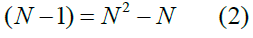
where P, the number of populations, P = N, and add the group size g in Eq. 2 to yield the total number of connections ctot, which is the population/ group cross-product in Fig. 1 minus the population/group blocks along the main diagonal:

Since, as mentioned, to keep the model simple but represent an approximate realistic network density in the brain, each neuron connects to 40% of all possible target neurons. Thus, network density is 40% in all experiments.

Experimental setup and neural simulation software

The effect of numbers of nodes and redundancy in connectivity between neural groups and the ‘robustness’ of the circuit and its output in terms of firing rates of the neurons as a whole is our focus. We explore robustness in neural circuits [1] using biologically-based modeling software that permits arbitrarily large numbers of unique neurons in terms of 10 membrane parameters and electrotonic dendritic connectivity, axonal projections to multiple synaptic locations with axonal delays, timesteps of 0.25 ms, and tracking of every synaptic event and membrane voltage at every time step [37,41]. With this more biologically-based representation of neural circuitry dynamics, we can rigorously control neuron numbers, connectivity, balance excitation and inhibition, and numbers of synapses as we manipulate the parameter space and sweep through a variety of sensitivity analyses. We use this ability to examine more closely the transition from less robust to more robust states and the relationship to the complexity of the network.

We prepared a baseline circuit as a configuration of 10-parameters and topology in the Universal Neural Circuitry Simulator (UNCuS) [37]. Models contained 2 - 9 populations, each containing one excitatory and one inhibitory neural group. Therefore, we examined fully interconnected circuits of balanced excitation and inhibition. To aid transparency and avoid confounding effects, parameters in only population #2 were varied and the firing rate of only one population, #1, was used to gauge variation of the network response.

Circuit Structure and Complexity Metrics

Connectivity parameters and calculations: Let us consider the connections between neurons in any two groups within the network. Each connection is one-way, commonly called a projection, and in the neural simulator there is only a single projection between any two groups, but each projection can connect any one neuron to any number of neurons in the target group (as a real axon might make several synapses on multiple target cells). The total number of axonal projections in the network then is:

Where,

p = number of populations in the network; gtot = total number of groups in the network, and gtot = 2 x p.

The connection ‘density’ of all cells in each group in the network is 40%, i.e., a projection consists of a pre-synaptic neuron randomly connecting to 40% post-synaptic neurons in the target group. Thus:

Where,

ccpost = number of connected target cells for a pre-synaptic cell and cpost = number of post-synaptic cells. Each projection contains connections = g size × ccpost, yielding a total number of connections in the network:

The synapses of each cell are made on an electrotonic space of 10 compartments that are, in terms of electrical resistance and therefore the current they send to the cell body when stimulated, able to simulate any arbitrary passive-resistance dendritic configuration [37,40], and numbered 1 - 10 from strongest to weakest effect on the axon hillock area of the cell.

Moreover, synapses further away, electrotonically, rise to a lower current amplitude but have a longer effect in time, whereas those closer to the cell body or axon hillock, electrotonically, have a much higher amplitude effect, but last a shorter time. Such dynamic dendritic processing provides a much richer representation of real dendritic processing than most neural network models and neural node models that use integrate-and-fire equations. If the number of dendritic compartments contacted in each target cell is 6 in all groups, for instance, then the total number of synapses in the entire network is given by:

To calculate the total complexity in the network incorporating that of all systems levels including number of cells, number of projections, and number of synapses, - the “combined complexity” C - is given by:

Where ctot = total number of cells in the network, i.e., ctot = gtot X g size.

Limitation: Randomized, non-clustered networks

All networks were randomized and homogenously connected, therefore, there were no ‘clusters’ i.e., highly connected nodes whose behavior might have a stronger effect on the rest of the network relative to that of other nodes. Connection density was uniform throughout the entire network and therefore a limited factor in examining local effects on a single group of neurons.

Metrics

Firing Rate (FR): Firing rate (FR) of each individual neuron, as it differs from a baseline to a value when the network is perturbed, is the single measure used in the two metrics describing network robustness. The momentary firing rate FR(t), where t is a given 0.25 ms time step, is calculated by averaging the number of spikes in the trailing 100 ms-period over all cells in a group:

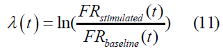
Robustness Metrics: Coefficient of Variance (CV) and Lyapunov Exponent (λ): Two measures of ‘robustness’ were used in this study, a variance metric, coefficient of variance (CV), and a type of Lyapunov exponent λ [42-47].

Coefficient of Variance (CV): The formula we used for coefficient of variance is given by:

Where σ is standard deviation; the middle expression shows that CV is a variance measure that uses some value of a baseline case as its unit, which in our study is the firing rate, FR. Intuitively, the smaller the variance CV from the baseline firing rate FRb of each network, the more robust the network and its tendency to maintain a ‘healthy’ state (see Discussion). In dynamical systems, intuitively, a Lyapunov exponent measures how rapidly two trajectories diverge from initial conditions in phase space. ‘Chaotic’ systems are defined as those that diverge rapidly from close initial points in the phase space. In this sense, robustness, as used herein, intuitively means less divergence between two transitions in phase space when their initial conditions are tweaked.

Lyapunov Exponent (λ): The formula we used for Lyapunov exponent is given as:

Measuring the critical point of a homeostatic healthy state vs. diseased state

Curve-fitting: The best-fit function (ExpDec1, OriginLab, Northampton, MA, USA) for the data was:

(12)

For which fitting coefficients are given in Table 2.

Identifying the transition toward greater stability: A question to consider with these curves, which can be interpreted as the transition from instability to robustness or to a homeostatic healthy state from a diseased or disordered state, is: At what point does such a transition take place? One method to determine this transition point is to use the point of maximum curvature, which is equivalent to the maximum speed of rotation of the tangent of the curve, as the critical transition point of the best-fit function. The procedure is then to find the minimum radius of curvature along the fitted curve. This point is located at:

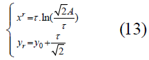
for which the derivation is given in the Supplement.

Analysis of increasing perturbation to disrupt stability: We also examined how much perturbation might be needed to move an otherwise robust network out of stability. With nine fully-interconnected populations of neurons at the highest connectivity (i.e., the most complex circuit), we manipulated parameters of the neurons in increasing numbers of populations and measured the CV to determine how much perturbation might disrupt the overall stability of the firing rate of neurons in group one.

Sensitivity testing

There are 10 neural cell membrane parameters used in UNCuS and each parameter has a fixed default value (Table S3) with slight jitter to make each cell unique. Running a given network with the default set reproduces a set of calibration data. To test sensitivity of a neural circuit to each parameter, we set each parameter to its default value as its baseline and assign random values to all other parameters within an assigned range (Table S3). This was done to assure that we had considered whether one or another parameter had more effect on circuit perturbation. When using firing rate FR as sensitivity metric, the FR variance, Vij, of a sample set was calculated as:

Where FRb is the firing rate with all 10 cell parameters are at their baseline values normalized by setting it equal to 1, i is the index of the randomly-selected cell parameter and j is the index of the sample set. Then the sensitivity of the ith cell parameter using sample set j was calculated as:

Experiment descriptions

Experiment 1: Variation of cell parameters, numbers of populations and groups: In the experiments, several levels of complexity were varied in cell behavior parameters, numbers of cells/group. A baseline case was created by using the default cell parameters given in Table A3. Stimulation was run for 1 second and the firing rates and robustness metrics were calculated for population 1 only. Tables S5 and S6 summarize experiments 1 and 2. In the third experiment, we tested the sensitivity of robustness against changes in 10 individual neuron parameters. Sensitivity was defined as the system’s average firing rates’ distance from its firing rate with the baseline parameters. The baseline firing rate was set at 1 to normalize rates for comparison.

Results

Experiment 1

Main result: Figure 3 shows that as complexity increases in circuits having different levels of complexity, the CV approaches an asymptotic value, (~0.26), and the most complex system has the slowest transition from a less robust to more robust state. The fitting parameter values are listed in Table 2 and coordinates of minimum curvature points are in Table 3. The CV of all four curves approaches an asymptote at ~0.26 (Eq. 9) instead of 0 because the deviation is relative to the baseline firing rate which itself is a function of the baseline parameter set of neuron parameters (Table S3). Importantly, however, is that as the systems become more complex, the CV reaches a fundamental lowest level compared to the baseline parameters. Looking at combined-complexity, robustness reaches its critical turning point at ~105.426 (266,686 total complexity in the circuit - neurons x projections x synapses), which corresponds to parameters of 2 populations with 5 cells in each group (Figure 3a). Of the four levels of complexity, the combined complexity radius of minimum curvature radius is greatest, (at value of 3.5), which implies that the transition from less to more robust is slower than in the less complex samples As complexity increases from total cells to total projections to total synapses to combined complexity, robustness, as measured by inverse of the coefficient of variation, increases (Table 2). The same data show that the more complex the system, the less rapid is its transition from less to more robust. Figure 4 shows a similar result as Figure 3, but for CV vs. network degree. Interestingly, as measured by the center of maximum curvature, the critical point toward robustness is 102.186, which is ~153 network connections. The fitting parameter values and coordinates of minimum curvature points are listed in Table 4.

Experiment 2

Main result: When the number of perturbed populations increases, the asymptote of robustness y0 increases as measured by average Lyapunov exponent, due to greater variability in the parameter space, while in all cases robustness increased with complexity Figure 5. The transition from less robust to more robust behavior can be seen along the perturbed population axis.

To examine how perturbation affects network stability, we set up 8 different stimulating population cases among 9 populations, using firing rate FR(t) in population 1 as the degree of perturbation and perturbations of cell parameters in successive subsets of populations 2-9 as the perturbation source (i.e., population 2, then populations 2 & 3, etc. up to populations 2-9). All other variables in the experiment are the same as in Experiment 1. The eight population perturbation runs are shown in Figure 5.

Figures 6 and 7 show robustness in the same setup using a different measure of stability, average Lyapunov Exponent (ALE). This measure, more closely related to typical LE analyses of dynamical systems to determine how quickly they diverge or converge as a measure of stability, shows that the dynamic ALE not only rapidly settles to the low positive value (~0.1) as complexity increases, but the standard deviation of its value decreases significantly as complexity increases. These findings are consistent with the changes seen at similar complexity values with CV measures. However, Fig. 6 shows that as ALE values are separated out for each level of complexity, it reveals itself to be less sensitive as a measure of robustness than CV in firing rate.

Experiment 3

Main result: Sensitivity was defined as the system’s average firing rates’ distance from its firing rate with baseline parameters, and that rate was set at 1 to normalize the plot (Eqs.13, 14 and 15). The network’s sensitivity to neuron parameter changes did not change with increased complexity Figure 8. Not unexpectedly, since we used firing rate as a metric for robustness, results were most sensitive to the baseline cell threshold, STh, than to any other parameter, since threshold directly modulates firing rate (firing rate is inversely proportional to threshold). Extensive examinations of the cell parameter space [48] reveal numerous stable attractors that are known as different types of neurons, which the nervous system has evolved to perform specific functions.

Discussion

Main results

Highly inter-connected and recurrent neural circuits throughout the CNS must be able to be perturbed by constant stimuli such as sensory input, to tolerate component failure, and yet be able to maintain function from an information processing standpoint, related primarily to firing patterns [45,49-51]. The main result of the first two experiments is that, given neural circuitry with a basic excitatory/inhibitory balance to remove that obvious known stability pre-requisite, robustness can be enhanced by increasing system complexity beyond a critical point [17,52].

Conversely, recurrence can be a source of instability and fragility when functioning as positive feedback but a source of stability and robustness when functioning as negative feedback [38,53-55]. Inherent ‘noise’ levels in a neural circuit may also be mechanisms of maintaining robustness [56], and the work herein shows that robustness against noise can emerge with increased complexity. These results may not apply to small, highly specific circuits [20]. But on the other hand, medium- to large-scale connectome models may require an inherent degree of complexity, visualized on the plots as a corner point at the minimum radius of curvature, to perform a variety of behaviors (input-output specifications) with character that is robustly like the actual system being portrayed. One conclusion that may apply to the evolution of neural circuits and more broadly to developing control systems or homeostatic systems is that, once a certain degree of complexity is in place, the system can evolve and perform robustly enough to contribute to a positive evolutionarilyselective force.

Addressing criticism of biological models

A criticism leveled against modeling in neural circuitry function has been that because all the neuron, ion channel, membrane parameter, transmitter, and ultrastructural components are typically not perfectly known, parameter wiggle room can be used to manipulate model behavior. One answer to this criticism is that as the system grows in complexity, the variation in any one parameter, or even several parameter values, may have diminishing impact on the overall stability and resulting system dynamics. Thus, manipulating individual parameters in localized parts of a circuit to bias it toward a desired outcome is unlikely to be effective unless significant numbers of parameters are changed in several areas or non-biological changes are made in some individual parameters.

As a corollary, when some parameters in a simulation are not precisely known but are estimated within a biologically reasonable range, the output of the circuit may nonetheless be similar to output when those parameters are precisely known And when modeling a nonlinear system with wide parameter ranges or ‘sloppy’ parameters, increasing model complexity may be a technique to help produce falsifiable predictions [57-59].

Rationale for using firing rate as the measure of variance

A significant advance on Bernard and Cannon’s homeostasis concept was made by the mathematician Norbert Wiener, who made homeostasis the centerpiece of his version of control theory, cybernetics. Cybernetics was conceived to bridge the gap between biological systems and autonomous systems that he envisioned would eventually lead to artificial general intelligence [60,61]. From a different perspective, functional connectivity is defined as correlation of activity between neural groups. “Activity” is measured in different ways that are all proxies for firing rates. Functional connectivity has grown in importance as a way to establish a baseline healthy state via the brain’s resting state functional connectivity, deviation from the healthy state, and restoration toward the healthy state by a given intervention [32,62-81].

Limitations

This study attempted to analyze the connectivity complexity in simplified, generic neural circuits. In the brain or spinal cord of most complex organisms, there are specific circuits that enable the enormous range of behaviors seen and any isolated part of that circuitry is not totally balanced by excitation and inhibition, numbers of synapses, and so forth. While we have tried to eliminate such connectivity as a factor in studying whether complexity per se creates robustness, we may have missed the transition points, earlier or later, in whether certain smaller or differently connected circuits could achieve robustness.

Moreover, disorders of neural circuitry physiology occur, such as seizure or movement disorder. Although such states could be seen as dysfunctional ‘stable attractor states’ of the system, they likely represent situations where cell parameter changes have strayed outside of a range we have considered. We did not attempt to account for diseased states categorized in terms of dynamical systems theory. A large part of the maintenance of membrane, synaptic, and circuitry parameters in real nervous systems are done by glia. Glia outnumber neurons by 10-20:1, communicate with each other and with neurons by gap junctions, and modulate neurotransmitters and other molecules affecting neural activity. Glia are a buffer for eliminating perturbed parameters and contribute to circuit robustness, but whose functions were not separated out in our study.

Conclusion

An analysis of biologically-based neural circuitry models, balanced in basic dimensions such as inhibition and excitation, shows that, with increasing complexity in numbers of elements, these systems become more robust and less sensitive to one or more parameter values. An evolutionary strategy to achieve robustness of desired behavior at multiple systems levels is to evolve component and connectivity properties that exceed critical values. These properties are independent of, and orthogonal to, redundancy alone and deserve study as a critical ingredient in biological homeostasis and the control theory of biological systems. As measured by the center of maximum curvature, the transition of the neural circuitry systems modeled was ~153 network connections (network degree).

Acknowledgment

Generous support for this work was provided by the Sydney Family Foundation. We thank K. Carlson for feedback and help with the manuscript.

Authorship Statement

JEA conceived and guided the simulations that LZ performed and from which the figures were selected. All authors researched the literature. K. Carlson helped to draft the paper, to which all authors contributed and approved.

Additional Information

The authors declare no competing interests.

References

1. Makarov, Sergey N., Gregory M. Noetscher and Aapo Nummenmaa. "Brain and HUMAN BODY MODEling 2020: computational human models presented at EMBC 2019 and the BRAIN Initiative® 2019 meeting."  407 (2021).

Google Scholar, Crossref, Indexed at

2. Ardesch, Dirk Jan, Lianne H. Scholtens and Martijn P. Van Den Heuvel. "The human connectome from an evolutionary perspective." Prog Brain Res 250 (2019): 129-151.

Google Scholar, Crossref, Indexed at

3. Bernard, Claude. Lectures on the phenomena of life common to animals and plants. Translation by Hebbel E. Hoff, Roger Guillemin [and] Lucienne Guillemin. (1974).

Google Scholar  

4. Cannon, Walter B. "Physiological regulation of normal states: Some tentative postulates concerning biological homeostatics." Paris: Editions Medicales. (1926).

Google Scholar, Crossref  

5. Demongeot, J., and L. Demetrius. Complexity and stability in biological systems. Intl J Bifurc Chaos 25 (2015).

Crossref, Indexed at

6. Wu, Yangle, Xiaomeng Zhang and Jianglei Yu, et al. "Identification of a topological characteristic responsible for the biological robustness of regulatory networks." PLoS Comput Biol 5 (2009): e1000442.

Google Scholar, Crossref, Indexed at

7. Eloundou-Mbebi, Jeanne M.O., Anika Küken and Nooshin Omranian, et al. "A network property necessary for concentration robustness." Nat Commun 7 (2016): 1-7.

Google Scholar, Crossref, Indexed at

8. Elton, Charles S. The ecology of invasions by animals and plants. Springer Nature, 2020.

Google Scholar, Crossref, Indexed at

9. Lomeli, Naomi, Daniela A. Bota and Kelvin J.A. Davies. "Diminished stress resistance and defective adaptive homeostasis in age-related diseases." Clin Sci 131 (2017): 2573-2599.

Google Scholar, Crossref, Indexed at

10. Pomatto, Laura C.D., and Kelvin J.A. Davies. "The role of declining adaptive homeostasis in ageing." J Physiol 595 (2017): 7275-7309.

Google Scholar, Crossref, Indexed at

11. Pomatto, Laura C.D. and Kelvin J.A. Davies. "Adaptive homeostasis and the free radical theory of ageing." Free Radic Biol Med 124 (2018): 420-430.

Google Scholar, Crossref, Indexed at

12. Pomatto, Laura C.D., Patrick Y. Sun and Kelvin J.A. Davies. "To adapt or not to adapt: Consequences of declining adaptive homeostasis and proteostasis with age." Mech Ageing Dev 177 (2019): 80-87.

Google Scholar, Crossref, Indexed at

13. Pomatto, Laura C.D., Patrick Y. Sun and Kelsi Yu, et al. "Limitations to adaptive homeostasis in an hyperoxia-induced model of accelerated ageing." Redox Biol 24 (2019): 101194.

Google Scholar, Crossref, Indexed at

14. Castaneda, E., Ian Q. Whishaw and Terry E. Robinson. "Changes in striatal dopamine neurotransmission assessed with microdialysis following recovery from a bilateral 6-OHDA lesion: variation as a function of lesion size." J Neurosci 10 (1990): 1847-1854.

Google Scholar, Crossref, Indexed at

15. Neumann, John Von. "Probabilistic logics and the synthesis of reliable organisms from unreliable components." Automata Stud 34 (1956): 43-98.

Google Scholar, Crossref, Indexed at

16. Barkai, Naama and Stan Leibler. "Robustness in simple biochemical networks." Nature 387 (1997): 913-917.

Google Scholar, Crossref, Indexed at

17. Ay, Nihat and David C. Krakauer. "Geometric robustness theory and biological networks." Theory Biosci 125 (2007): 93-121.

Google Scholar, Crossref, Indexed at

18. Cohen, Reuven, Keren Erez and Daniel Ben-Avraham, et al. "Resilience of the internet to random breakdowns." Phys Rev Lett 85 (2000): 4626.

Google Scholar, Crossref, Indexed at

19. Doyle, John C., David L. Alderson and Lun Li, et al. "The “robust yet fragile” nature of the Internet." Proc Natl Acad Sci 102 (2005): 14497-14502.

Google Scholar, Crossref, Indexed at

20. Alcalde Cuesta, Fernando, Pablo Gonzalez Sequeiros and Alvaro Lozano Rojo. "Exploring the topological sources of robustness against invasion in biological and technological networks." Sci Rep 6 (2016): 1-13.

Google Scholar, Crossref, Indexed at

21. Xu, Ting, Karl-Heinz Nenning and Ernst Schwartz, et al. "Cross-species functional alignment reveals evolutionary hierarchy within the connectome." Neuroimage 223 (2020): 117346.

Google Scholar, Crossref, Indexed at

22. Lorenz, Edward N. "A new approach to linear filtering and prediction problems." Deterministic Nonperiodic flow 20 (1963): 130-141.

Google Scholar, Crossref, Indexed at

23. Green, June Barrow. "Poincaré and the three body problem providence, RI." Amer Math Soc (1996).

Google Scholar

24. Hu, Jin and Jun Wang. "Global stability of complex-valued recurrent neural networks with time-delays." IEEE Trans Neural Netw Learn Syst 23 (2012): 853-865.

Google Scholar, Crossref, Indexed at

25. Barkai, Naama and Ben-Zion Shilo. "Variability and robustness in biomolecular systems." Mol Cell 28 (2007): 755-760.

Google Scholar, Crossref, Indexed at

26. Song, Xueli, Xing Xin and Wenpo Huang. "Exponential stability of delayed and impulsive cellular neural networks with partially Lipschitz continuous activation functions." Neural Netw 29 (2012): 80-90.

Google Scholar, Crossref, Indexed at

27. Kunert, James M., Pedro D. Maia and J. Nathan Kutz. "Functionality and robustness of injured connectomic dynamics in C. elegans: linking behavioral deficits to neural circuit damage." PLoS Comput Biol 13 (2017): e1005261.

Google Scholar, Crossref, Indexed at

28. Hu, Jin and Jun Wang. "Global exponential periodicity and stability of discrete-time complex-valued recurrent neural networks with time-delays." Neural Netw 66 (2015): 119-130.

Google Scholar, Crossref, Indexed at

29. Sandler, U., and L. Tsitolovsky. "The S-Lagrangian and a theory of homeostasis in living systems." Phys A: Stat Mech Appl 471 (2017): 540-553.

Google Scholar, Crossref, Indexed at

30. Demongeot, Jacques, Eric Goles and Michel Morvan, et al. "Attraction basins as gauges of robustness against boundary conditions in biological complex systems." PloS One 5 (2010): e11793.

Google Scholar, Crossref, Indexed at

31. Anafi, Ron C., and Jason H.T. Bates. "Balancing robustness against the dangers of multiple attractors in a Hopfield-type model of biological attractors." PLoS One 5 (2010): e14413.

Google Scholar, Crossref, Indexed at

32. Paul, Subhadip, Aditi Arora and Rashi Midha, et al. "Autistic traits and individual brain differences: Functional network efficiency reflects attentional and social impairments, structural nodal efficiencies index systemising and theory-of-mind skills." Mol Autism 12 (2021): 1-18.

Google Scholar, Crossref, Indexed at

33. Loh, Marco, Edmund T. Rolls and Gustavo Deco. "A dynamical systems hypothesis of schizophrenia." PLoS Comput Biol 3 (2007): e228.

Google Scholar, Crossref, Indexed at

34. Rolls, Edmund T., Marco Loh and Gustavo Deco. "An attractor hypothesis of obsessive–compulsive disorder." Eur J Neurosci 28 (2008): 782-793.

Google Scholar, Crossref, Indexed at

35. Fornito, Alex, Andrew Zalesky and Edward Bullmore. Fundamentals of brain network analysis. Academic Press, 2016.

Google Scholar 

36. Sporns, Olaf. "Structure and function of complex brain networks." Dialogues Clin Neurosci (2022).

Google Scholar, Crossref, Indexed at

37. Arle J.E, L.Z. Mei and J.L. Shils. "Modeling Parkinsonian circuitry and the DBS electrode." Stereotact Funct Neurosurg 86 (2008): 1-15.

Google Scholar, CrossrefIndexed at

38. Arle Jeffrey E., Nicolae Iftimia, Jay L. Shils and Longzhi Mei, et al. "Dynamic computational model of the human spinal cord connectome." Neural Comput 31 (2019): 388-416.

Google Scholar, Crossref, Indexed at

39. Fransson, Peter and William H. Thompson. "Temporal flow of hubs and connectivity in the human brain." Neuroimage 223 (2020): 117348.

Google Scholar, Crossref, Indexed at

40. Rall and Wilfrid. "Electrophysiology of a dendritic neuron model." Biophys J 2 (1962): 145.

Google Scholar, Crossref, Indexed at

41. Lyapunov, Aleksandr Mikhailovich. "The general problem of the stability of motion." Int J Control 55 (1992): 531-534.

Google Scholar, Crossref, Indexed at

42. Barreira, Luis and Claudia Valls. "Stability of the Lyapunov exponents under perturbations." Ann Funct Anal 8 (2017): 398-410.

Google Scholar, Crossref, Indexed at

43. Pikovsky, Arkady and Antonio Politi. Lyapunov exponents: a tool to explore complex dynamics. Cambridge University Press, 2016.

Google Scholar 

44. Chambers, Anna R., and Simon Rumpel. "A stable brain from unstable components: Emerging concepts and implications for neural computation." Neuro sci 357 (2017): 172-184.

Google Scholar, Crossref, Indexed at

45. Ozcan, Neyir and Sabri Arik. "Global robust stability analysis of neural networks with multiple time delays." IEEE Trans Circuits Syst I Regul Pap 53 (2006): 166-176.

Google Scholar, Crossref, Indexed at

46. Faydasicok, Ozlem and Sabri Arik. "Robust stability analysis of a class of neural networks with discrete time delays." Neural Netw 29 (2012): 52-59.

Google Scholar, Crossref, Indexed at

47. Arle and Jeffrey Edward. "Neural modeling of the cochlear nucleus." PhD diss., University of Connecticut, 1992.

Google Scholar

48. Mason, Paul H., Bodo Winter and Andrea Grignolio. "Hidden in plain view: degeneracy in complex systems." Biosyst  128 (2015): 1-8.

Google Scholar, Crossref, Indexed at

49. Kaluza, Pablo, Martin Vingron and Alexander S. Mikhailov. "Self-correcting networks: Function, robustness, and motif distributions in biological signal processing." Chaos: An Interdisciplinary J Nonlinear Sci 18 (2008): 026113.

Google Scholar, Crossref, Indexed at

50. Feala, Jacob D., Jorge Cortes and Phillip M. Duxbury, et al. "Statistical properties and robustness of biological controller-target networks." PloS one 7 (2012): e29374.

Google Scholar, Crossref, Indexed at

51. Lehár, Joseph, Andrew Krueger and Grant Zimmermann, et al. "High‐order combination effects and biological robustness." Mol Syst Biol 4 (2008): 215.

Google Scholar, Crossref, Indexed at

52. Wang and Xiao-Jing. "Decision making in recurrent neuronal circuits." Neuron 60 (2008): 215-234.

Google Scholar, Crossref, Indexed at

53. Khammash and Mustafa. "An engineering viewpoint on biological robustness." BMC Biol 14 (2016): 1-11.

Google Scholar, Crossref, Indexed at

54. Kwon, Yung-Keun and Kwang-Hyun Cho. "Quantitative analysis of robustness and fragility in biological networks based on feedback dynamics." Bioinformatics 24 (2008): 987-994.

Google Scholar, Crossref, Indexed at

55. Olin-Ammentorp, Wilkie, Karsten Beckmann and Catherine D. Schuman, et al. "Stochasticity and robustness in spiking neural networks." Neurocomput 419 (2021): 23-36.

Google Scholar, Crossref, Indexed at

56. Gutenkunst, Ryan N., Fergal P. Casey and Joshua J. Waterfall, et al. "Extracting falsifiable predictions from sloppy models." Ann N Y Acad Sci 1115 (2007): 203-211.

Google Scholar, Crossref, Indexed at

57. Berro, J. "Essentially, all models are wrong, but some are useful"-a cross-disciplinary agenda for building useful models in cell biology and biophysics. Biophys Rev 10(2018:1637-47.

Crossref, Indexed at

58. Gutenkunst R.N, Waterfall J.J, Casey F.P and Brown K.S, et al. Universally sloppy parameter sensitivities in systems biology models. PLoS Comp Bio 3(2007):1871-78.

Crossref, Indexed at

59. Wiener and Norbert. The human use of human beings: Cybernetics and society. No. 320. Da Capo Press, 1988.
60. Russell and Stuart. Human compatible: Artificial intelligence and the problem of control. Penguin, 2019.

Google Scholar

61. Wang, Zhijiang, Zhengjia Dai and Gaolang Gong, et al. "Understanding structural-functional relationships in the human brain: A large-scale network perspective." The Neuroscientist 21(2015): 290-305.

Google Scholar, Crossref, Indexed at

62. Furman, Daniella J., J. Paul Hamilton and Ian H. Gotlib. "Frontostriatal functional connectivity in major depressive disorder." Biol Mood Anxiety Disord 1 (2011): 1-11.

Google Scholar, Crossref, Indexed at

63. Schlee, Winfried, Vera Leirer and Iris-Tatjana Kolassa, et al. "Age-related changes in neural functional connectivity and its behavioral relevance." BMC Neurosci 13 (2012): 1-11.

Google Scholar, Crossref, Indexed at

64. Davis, Karen D., and Massieh Moayedi. "Central mechanisms of pain revealed through functional and structural MRI." J Neuroimmune Pharmacol 8 (2013): 518-534.

Google Scholar, Crossref, Indexed at

65. Little, Simon, Huiling Tan and Anam Anzak, et al. "Bilateral functional connectivity of the basal ganglia in patients with Parkinson’s disease and its modulation by dopaminergic treatment." PLoS One 8 (2013): e82762.

Google Scholar, Crossref, Indexed at

66. Bielza, Concha and Pedro Larranaga. "Bayesian networks in neuroscience: A survey." Front Comput Neurosci 8 (2014): 131

Google Scholar, Crossref, Indexed at

67. Chen, Li Min, Arabinda Mishra and Pai-Feng Yang, et al. "Injury alters intrinsic functional connectivity within the primate spinal cord." Proc Natl Acad Sci 112 (2015): 5991-5996.

Google Scholar, Crossref, Indexed at

68. Kaiser, Roselinde H., Susan Whitfield-Gabrieli and Daniel G. Dillon, et al. "Dynamic resting-state functional connectivity in major depression." Neuro Psycho Pharmacol 41 (2016): 1822-1830.

Google Scholar, Crossref, Indexed at

69. Gong, Liang, Yingying Yin, Cancan He and Qing Ye, et al. "Disrupted reward circuits is associated with cognitive deficits and depression severity in major depressive disorder." J Psychiatr Res 84 (2017): 9-17.

Google Scholar, Crossref, Indexed at

70. Barch, Deanna M. "Resting state functional connectivity in the human connectome project: Current Status and relevance to understanding psychopathology." Harv Rev Psychiatry 25 (2017): 209.

Google Scholar, Crossref, Indexed at

71. Amico, Enrico, Daniele Marinazzo and Carol Di Perri, et al. "Mapping the functional connectome traits of levels of consciousness." Neuroimage 148 (2017): 201-211.

Google Scholar, Crossref, Indexed at

72. Tinaz, Sule, Peter M. Lauro and Pritha Ghosh, et al. "Changes in functional organization and white matter integrity in the connectome in Parkinson's disease." NeuroImage Clin 13 (2017): 395-404.

Google Scholar, Crossref, Indexed at

73. Sharma, Anup, Daniel H. Wolf and Rastko Ciric, et al. "Common dimensional reward deficits across mood and psychotic disorders: a connectome-wide association study." Am J Psychiatry 174 (2017): 657-666.

Google ScholarCrossref, Indexed at

74. Bijsterbosch, Janine and Christian Beckmann. An introduction to resting state fMRI functional connectivity. Oxford University Press, 2017.

Google Scholar 

75. Chen, Li Min, Pai-Feng Yang and Feng Wang, et al. "Biophysical and neural basis of resting state functional connectivity: Evidence from non-human primates." Magn Reson Imaging 39 (2017): 71-81.

Google Scholar, Crossref, Indexed at

76. Smitha K. A, K. Akhil Raja, K. M. Arun and P. G. Rajesh, et al. "Resting state fMRI: A review on methods in resting state connectivity analysis and resting state networks." Neuroradiol J 30 (2017): 305-317.

Google Scholar, Crossref, Indexed at

77. Ito, Takuya, Kaustubh R. Kulkarni and Douglas H. Schultz, et al. "Cognitive task information is transferred between brain regions via resting-state network topology." Nat Commun 8 (2017): 1-14.

Google Scholar, Crossref, Indexed at

78. Gilson, Matthieu, Nikos E. Kouvaris and Gustavo Deco, et al. "Network analysis of whole-brain fMRI dynamics: A new framework based on dynamic communicability." NeuroImage 201 (2019): 116007.

Google Scholar, Crossref, Indexed at

79. Shine, James M., Peter T. Bell and Elie Matar, et al. "Dopamine depletion alters macroscopic network dynamics in Parkinson’s disease." Brain 142 (2019): 1024-1034.

Google Scholar, Crossref, Indexed at

80. Ruppert, Marina C., Andrea Greuel and Masoud Tahmasian, et al. "Network degeneration in Parkinson’s disease: Multimodal imaging of nigro-striato-cortical dysfunction." Brain 143 (2020): 944-959.

Google Scholar, Crossref, Indexed at

81. Van Doremalen, Neeltje, Teresa Lambe and Alexandra Spencer, et al. "ChAdOx1 nCoV-19 vaccine prevents SARS-CoV-2 pneumonia in rhesus macaques." Nature 586 (2020): 578-582.

Google Scholar, Crossref, Indexed at