Research Article - (2023) Volume 12, Issue 1
Received: 13-Sep-2022, Manuscript No. jme-22-75322;
Editor assigned: 16-Sep-2022, Pre QC No. jme-22-75322 (PQ);
Reviewed: 30-Sep-2022, QC No. jme-22-75322;
Revised: 23-Dec-2022, Manuscript No. jme-22-75322 (R);
Published:
03-Jan-2023
, DOI: 10.37421/jme.2023.12.629
Citation: Altamimi, Ragai and El-Genk, Mohamed S (2023)
“Equivalent Circuit Model for Predicting the Performance Characteristics
of Direct Current-Electromagnetic Pumps”. J Material Sci Eng 12 (2023):629.
Copyright: © 2023 Altamimi R, et al. This is an open-access article
distributed under the terms of the Creative Commons Attribution License,
which permits unrestricted use, distribution, and reproduction in any
medium, provided the original author and source are credited.
Direct Current-Electro Magnetic Pumps (DC-EMPs) are passive with no moving parts for circulating liquid metals in industrial applications, nuclear reactors, and experimental test loops. The Equivalent Circuit Model (ECM) is easy to apply and has been widely used to evaluate the performance of DC-EMPs. It over predicts the pumping pressure and the pump characteristics due to the incorporated assumptions. teffective magnetic flux density. This work quantifies the effects of these assumptions on the ECM predictions for a mercury DC-EMP. Analyzed experimental measurements for this pump show the fringe resistance and the magnetic flux density are not constant but depend on those of the liquid flow rate and the input electrical current. Results show that the 2D Finite Element Method Magnetics (FEMM) software accurately predicts the obtained values of the fringe resistance and the magnetic field flux density from the reported measurements at zero flow for use in ECM. With these values and the measured wall electrical contact resistance, the ECM over predicts the measured characteristics of the mercury pump by only ~7%. Neglecting the wall electrical contact resistance causes the ECM to over predict the pumping pressure for the mercury DC-EMP at an input electrical 6,740 A by 0.2-1.4%, depending on the flow rate. Nonetheless, accounting for the dependences of the fringe resistance and the magnetic flux density on the input electrical current and the liquid flow rate is important to accurately predicting the performance of DC-EMP, which is not possible using the ECM.
DC electromagnetic pump • Equivalent circuit model • Mercury pump experimental characteristics • Fringe resistance • Magnetic flux density • Finite Element Method Magnetics.
a Pump duct width (m)
A Duct flow area (m2)
AUV Autonomous Underwater Vehicle
B Pump duct height (m)
B Magnetic flux density (T)
Bo Magnetic flux density at zero flow (T)
 Effective magnetic flux density at zero flow (T)
C Pump duct length (m)
DC-EMP Direct Current-Electromagnetic Pump
De Duct equivalent hydraulic diameter (m)
 Pump terminal voltage (V)
Ei Induced emf (V)
ECM Equivalent Circuit Method
Emf Electromotive force (V)
F Force (N)
 Pump input current (A)
Ie Pump effective current (A)
Ieo Pump effective current at zero flow rate (A)
IFEMM FEMM input current (A)
If Fringe current (A)
Ifo Fringe current at zero flow rate (A)
Iw Duct wall current (A)
 Current density (A/m2)
K1 Fringe correction factor
MHD Magneto hydrodynamic
FEMM Finite Element Method Magnetics
 Pressure (Pa)
Ploss Hydraulic pressure losses (Pa)
PO Static pumping pressure (Pa)
Pp Developed pumping pressure (Ω)
 Volumetric flow rate (m3/s)
Re Working fluid electrical resistance in pump region (Ω)
Rf Fringe electrical resistance (Ω)
Rf o Fringe electrical resistance at zero flow
Rstat Static electrical resistance (Ω)
RW Wall electrical resistance (Ω)
SRPS Space Reactor Power System
e Effective
f Fringe
p Pump
w Wall
wf Working fluid
 Thickness (m)
 Pump efficiency (%)
 Dynamic viscosity (Pa.s)
ρ Density (kg/m3), Electrical resistivity (Ω.m)
Direct Current-Electromagnetic Pumps (DC-EMPs) drive the flows of liquid metals and electrically conductive liquids in industrial, biological, and solar energy applications [1-3], and for cooling terrestrial and space nuclear reactor power systems [4,5]. Liquid metals of interest include molten lead, leadbismuth alloy, aluminum, bismuth, gallium, sodium, lithium, and sodiumpotassium alloys [6-8]. These liquid metals span a wide range of thermal and physical properties, including the melting point, density, dynamic viscosity, specific heat capacity, thermal conductivity, magnetic permeability, and electric resistivity. DC-EMPs Passively drive these electrically conductive liquids by the Lorentz force generated by passing a direct electrical current through the liquid in the perpendicular direction of an applied magnetic field. These pumps require low terminal voltage (<2 VDC) and hundreds to thousands of amperes of electrical current. A permanent magnet operating sufficiently below the Curie point, or an electromagnet that requires electric power for its operation, will provide the magnetic flux density [10-11]. The permanent magnet DC-EMPs are a preferable choice for Space Nuclear Reactor Power Systems (SRPSs) with static thermoelectric (TE) or thermionic (TI) energy conversion modules [4,9]. Besides being fully passive with no moving parts they facilitate the safe removal of the decay heat generated in the nuclear reactor after shutdown. In these power systems, dedicated energy conversion modules provide the electrical current to the pump during nominal operation and after shutdown. In addition to the design simplicity, absence of moving parts, limited maintenance, and high reliability the permanent magnet DC-EMPs are typically smaller in size and lighter than electromagnets DC-EMPs [12-14].
The performance characteristics of DC-EMPs depend on the liquid properties and temperature, the dimensions and wall materials of the flow duct, the magnet material and the value of the magnetic flux density, and the values of the input electric current and fringe resistance [15-17]. These design and performance parameters are typically based on direct experimental measurements. However, for new pump designs with desired specific operation and performance requirements direct measurements are not possible a priori.
Instead, the electrical Equivalent Circuit Method (ECM) can help develop a preliminary pump design and predict the performance characteristics. The wide use of the ECM is because of its simplicity despite incorporating simplifying assumptions that result in over predicting the pump performance [6,10]. These include assuming constant fringe resistance, constant and uniform magnetic field flux, and electrical current densities, neglecting the electrical contact resistance of the duct wall, and neglecting the dependences of the fringe resistance and magnetic flux density on the flow rate of the pumped liquid metals and input electrical current. The used values of the fringe resistance and the magnetic flux density in the ECM were either arbitrarily assumed or estimated using invalidated empirical relations [6,10,17].
Johnson [12] has designed and measured the performance of a DCEMP for circulating liquid NaK-78 working fluid and coolant for SRPSs. With limited direct measurements, he conducted performance analysis using the ECM. The analysis used the measured magnetic flux density in the pump duct at zero flow and an assumed fringe resistance based on previous experimental studies of DC-EMP of different geometries. Which are both assumed constant and independent of the input electrical current and liquid flow rate? For operating at 316°C and input current of 1,570 A, the ECM overestimated the static pressure at zero flow by ~15% and underestimated it by ~20% at a flow rate of ~2 kg/s, compared to the experimental measurements. These differences are due to uncertainties in the dimensions of the manufactured pump duct and an inaccurate estimate of the fringe resistance.
Nashine, et al. [10] used the ECM to investigate the performance of a DC-EMP design for circulating Sodium at 560°C in fast reactors auxiliary systems. The constructed and tested pump provided a pumping pressure of 176 kPa at an input electrical current of 2,000. Nashine et al. [10] used an empirical correlation proposed by Baker and Tessier [6] for calculating the fringe resistance in the performed analysis with the ECM. The ECM predictions of the pump characteristics were >40% higher than those measured. Post experiment analysis indicated that the suggested expression by Baker and Tessier overestimates the value of the fringe resistance by ~25%, contributing to overestimating the pump characteristics by >40%.
Umans, et al. [11] have used the ECM to help design and analyze the performance of a DC-EMP with u-shaped current electrodes for circulating Gallium in a power system for Autonomous Underwater Vehicles (AUVs). Their analysis neglected the fringe resistance and used a constant magnetic flux density value. The ECM predictions of the static pressure were ~2.6 times those measured. This difference is explained to be due to the shapes of the magnet and current electrode, which caused large non uniformities in the actual magnetic flux and the electric current densities in the tests. Measurements showed low current density exists in the regions of high magnetic flux density and vice versa.
Recently, Lee and Kim [16] designed a DC-EMP for circulating liquid sodium at 300°C in an experimental test loop. They used the ECM to perform parametric analyses of the pump dimensions to provide a pumping pressure of 5 kPa at sodium flow rate of 0.18 m3/hr. In their analyses, Lee, and Kim [16] used empirical correlation proposed by Baker and Tessier [6] to estimate the fringe resistance in the ECM analysis. They also performed 3D numerical analysis using ANSYS code to perform Magnetohydrodynamics (MHD) analysis of the pump characteristics. Results showed that calculated pumping pressure using MHD analyses at sodium flow rate 0.18 m3/hr of 4.3 kPa is ~52.4% of the predicted value using ECM (8.2 kPa). These results confirmed that contribution of the assumed values of the fringe resistance and the magnetic flux density in the ECM to over predicting the characteristics of the sodium DCEMP. The reported experimental measurements in the literature for the performance of DC-EMPs are either limited or incomplete for validating the ECM predictions [12,16]. Reported results showed the ECM over predict the performance characteristics of DC-EMPs by up to 40% [10].
In summary, due to its simplicity the ECM is widely used to evaluate the performance and predict the characteristics of DC-EMPs. However, due to the incorporated assumptions and arbitrary input values of the fringe resistance and the magnetic field flus density, the ECM overestimates the pump performance. These assumptions include neglecting the duct wall electrical contact resistance and using arbitrary constant input values of the fringe resistance and effective magnetic flux density and neglecting the effects of the input electrical current and the liquid flow rate. Therefore, it is desirable to quantify the effects of these assumptions on the predictions of the performance and characteristics of DC-EMPs, which requires experimental measurements or performing MHD analysis of the DC-EMP design of interest. Such an analysis is computationally intensive compared to using the ECM. The ECM can help in the development of a preliminary design or conduct approximate performance analysis of DC-EMPs using constant values of the fringe resistance and the magnetic field flux density that equal those at zero flow. This would require confirming a reliable approach for calculating these values, which is a focus of this work.
The objectives of the present work are to:
a. Analyze the reported experimental measurements for a mercury DC-EMP to determine the values of the fringe resistance and the magnetic flux density and their dependences on the liquid flow rate and the input electrical current [18];
b. Examine the accuracy of the 2D Finite Element Method Magnetics (FEMM) software of calculating the fringe resistance and the magnetic field flux density at zero flow for use in ECM;
c. Compare reported measurements of the mercury DC-EMP characteristic to the predictions of the ECM to quantify the effects of the various assumptions.
Operation Principle of DC-EMPs
A DC-EMP comprises of a small height rectangular duct for the flowing electrically conductive liquid, permanent or electromagnets on both sides of the flow duct, and electrodes for supplying electrical current (I) in the perpendicular directions to both the magnetic field and liquid flow (Figure 1). The coupling of the supplied electrical current, I, and the perpendicular magnetic flux density, B, in the pump duct generates “Lorentz” force, F, to derive the liquid flow in the perpendicular direction to the B x I plane [6,10]. The induced pressure rise across the pump duct, ΔP=F/(a x b) [19] depends on the dimensions of the flow duct, the values of magnetic flux density, the thermo physical and electrical properties and flow rate of the driven liquid metal and the operating temperature (Eq. 1) (Figures 2 and 3).

Figure 1. An illustration of the operation Principle of a DC-EMP.

Figure 2. Application of Fleming’s left-hand rule to Operation DC-EMP.

Figure 3. Cross-sectional views of a DC-EMP and an illustration of the electrical current component in a DC-EMP.
Ideal DC-EMP will have the supplied current (I) passing uniformly through the liquid within the flow duct, and the same for the magnetic flux density, however, this is not the case. The electric current (I) supplied by the electrodes is the sum of three parts, namely: (a) the effective current Ie that interacts with magnetic flux (B) to generate Lorentz force in the flow duct, (b) the current passing through the duct walls. The fringe currents flowing downstream and upstream of the duct region. The wall and fringe currents, (IW) and (If), do not contribute to the generation of the Lorentz force for driving the liquid metal flow through the pump duct. Similarly, only a fraction of the magnetic field flux density contributes to the generated Lorentz force in the flow duct of the pump [20-21]. The flow of the liquid in the duct in the perpendicular direction to the applied magnetic field induces an opposing electromotive force, emf (Ei), that reduces the effective current in the pump duct, Ie and increase the wall and fringe currents (Figure 4). The magnitude of induced emf, (Ei), depends on flow rate, magnetic flux density, and pump duct height [24].

Figure 4. DC-EMP equivalent electric circuit.
Electrical equivalent circuit model
Barnes [25] was the first to apply the Equivalent Circuit Model (ECM) for predicting the performance of DC-ECMS for circulating liquid sodium for cooling fast spectrum nuclear reactors. The ECM represents an equivalent circuit diagram for the pump (Figure 4). It includes the electrical resistances of the flow duct wall Rw, the fringe current flow, If, upstream and downstream of the pump duct, Rf, and of the coolant flowing through the pump duct, Re. The ECM also includes the induced opposing voltage, Ei, by the liquid metal flow in the pump duct. A current source provides the total current, I, to the pump electrodes at a terminal voltage, E. Eq. (1) below, expresses the developed pumping pressure for driving the liquid metal flow through the pump duct, ΔP, in terms of the applied magnetic field flux density, various resistances, the total electrical current, the height of the flow duct, b, and liquid metal volumetric flow rate, Q, as:
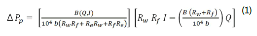
In this expression, ΔPp, is the developed pumping pressure across the
flow duct in Pa,  is the effective magnetic flux density in the pump
duct in Gauss,
is the effective magnetic flux density in the pump
duct in Gauss,  is the total electrical current supplied to the pump in
amperes (A),
is the total electrical current supplied to the pump in
amperes (A),  is the height of the pump duct in meters, and
  is the
volumetric flow rate of the liquid metal flow through the duct in m3/s. All
electrical resistances (Rw,Rf and Re ) in Eq. (1) are in Ohm (Ω).
is the
volumetric flow rate of the liquid metal flow through the duct in m3/s. All
electrical resistances (Rw,Rf and Re ) in Eq. (1) are in Ohm (Ω).
The net pumping pressure developing across the flow duct,  , after
accounting for the friction pressure losses, ΔPloss, of the flowing liquid
metal through the pump duct, is given as:
, after
accounting for the friction pressure losses, ΔPloss, of the flowing liquid
metal through the pump duct, is given as:

In the present analysis, the following expression [26] calculates the friction pressure losses, ΔPloss for the liquid flow in the pump duct, as:

In this expression, De is the flow duct equivalent hydraulic diameter in
meters, A is the duct cross-sectional flow area in m2,  is the duct length
in meters,
is the duct length
in meters,  is the density of the liquid in kg/m3,μ is the dynamic viscosity
of the liquid in Pa.s. For laminar flow, the coefficient “a” and the exponent
“b” equal 64 and 1.0, respectively, while for turbulent flow “a” and “b” are
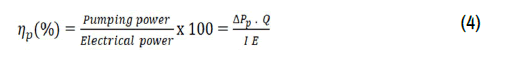
0.184 and 0.2, respectively [27]. The pump efficiency equals the net
pumping power divided by the input electrical power, as:
is the density of the liquid in kg/m3,μ is the dynamic viscosity
of the liquid in Pa.s. For laminar flow, the coefficient “a” and the exponent
“b” equal 64 and 1.0, respectively, while for turbulent flow “a” and “b” are
0.184 and 0.2, respectively [27]. The pump efficiency equals the net
pumping power divided by the input electrical power, as:
Eqs. (1)-(3) calculate the pump characteristics (ΔP versus Q) at different values of the magnetic flux density and the electrical current input, and in terms of the electrical properties of the duct wall and the flowing liquid. The electrical resistances of the duct wall and the liquid in terms of their electrical properties at the specified liquid temperature, and the values of B and Rf, which are functions of the liquid flow rate, Q, and the input current, I, need to be known a prior. Therefore, using ECM with simplifying assumptions, although easy and straightforward, over predicts the pump characteristics and performance parameters. These assumptions include constant and uniform distributions of I and B and neglecting the dependence of both B and Rf on the liquid flow rate, Q, and the supplied electrical current, I, as well as neglecting the contact electrical resistance of the duct wall. To quantify the effect of these assumptions, the present work compared the predicted pump characteristics using the ECM to the reported measurements for a mercury DC-EMP [18].
The next section describes the mercury DC-EMP designed and evaluated by Watt et al. [18]. It also presents and analyzes the reported experimental measurements and pump characteristics used to determine the values and the dependences of the magnetic flux density, B, and the Fringe resistance, Rf, on the liquid mercury flow rate, Q, and the input electrical current, I. It is worth noting that the values of the magnetic flux density and the fringe resistance at zero flow, Bo and Rfo, are independent of the input electrical current, I.
Mercury DC-EMP description and results
Watt et al. designed and constructed a DC-EMP for circulating liquid mercury in a test loop at room temperature. The pump had stainless steel duct and copper current electrodes. Electromagnets generate magnetic flux density in the pump duct. Laminated blocks extended the poles of the electromagnets beyond current electrodes to obtain a uniform distribution of the magnetic flux density in the liquid flow duct (Figure 5). This duct was 355 mm long, 152 mm wide, and 15.1 mm high and the duct wall was 0.6 mm thick. The supplied DC to the Cu electrodes varied from 1,980 to 10,400 A. Performed measurements included the electrodes’ terminal voltages, the magnetic flux density in the pump duct at zero flow, Bo, and the pumping pressure, ΔP, up to 300 kPa for circulating the liquid mercury in the test loop with 101.6 mm diameter piping at a volumetric flow rate, Q, up to ~26 m3/hr.

Figure 5. Extended electromagnet poles and the measured magnetic flux density along the effective duct length of the mercury DC-EMP [18].
Reported experimental measurements
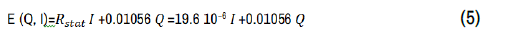
Watt et al. [18] measured the voltage difference across the pump duct at different electrodes currents and mercury circulation rates (Figure 6). The total static electrical resistance of the pump duct, Rstat, is determined from the measured terminal voltages at electrode currents ranging from 2,000-6,000 A, at zero flow, is ~19.6 μΩ. The static electrical resistance across the pump duct includes those of the duct wall, Rw, the fringe current, Rf, and the liquid mercury residing in the pump duct, Re (Figure 4). After draining liquid mercury from the pump duct the measured duct wall resistance was 230 μΩ. The reported experimental data displayed in Figure 6 shows the terminal voltage increases with increased electrode current and linearly at the same slope of ~0.01056 with an increased circulation rate of liquid mercury in the test loop. The reported measurements of the terminal voltage, E, in Figure 6 are correlated in the present work in terms of the measured values of static electrical resistance of the pump duct, Rstat, the input electrode current, I, and the flow rates of liquid mercury, Q, as:

Figure 6. Reported measurements of the terminal voltage at different electrode currents and circulation rate of liquid mercury [18].
Fringe resistance
Based on the pump equivalent circuit diagram in Figure 4, the following expression calculates the total fringe resistance for the mercury pump [18], as:
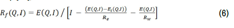
In Eq. (6), Ei (Q, I) is the induced opposing voltage in the pump duct due to the flow of liquid mercury in the applied magnetic field. The following expression calculates the induced voltage, Ei. It is zero when the liquid metal in the pump duct is stationary, Q=0, in terms of the magnetic flux density in the pump duct, B, and the duct height, b,

The obtained value of the total fringe resistance for the mercury DC-EMP
design [18] from the reported measurements at zero flow is 103.782  (Figure 7a). This value is independent of the supplied electrical current to
the electrodes (Figure 7). The results presented in this figure show that
the values of the total fringe resistance for the mercury DC-EMP [18]
increase almost logarithmically with increased mercury flow rate
(Figure 7a) and decrease almost linearly with increased electrical
current supplied to the pump’s electrodes (Figure 7b). The largest value
of the fringe resistance, Rf, for I=3970 A is only 4.3% higher than at value
at zero flow, Rfo(Figure 7). Therefore, using the fringe resistance in the
ECM equals that at zero flow (i.e., Rf=Rfo), and neglecting the changes
with the mercury flow rate and the electrodes current (Figure 7) cause the
ECM to under predict the pumping pressure by a few percentages.
(Figure 7a). This value is independent of the supplied electrical current to
the electrodes (Figure 7). The results presented in this figure show that
the values of the total fringe resistance for the mercury DC-EMP [18]
increase almost logarithmically with increased mercury flow rate
(Figure 7a) and decrease almost linearly with increased electrical
current supplied to the pump’s electrodes (Figure 7b). The largest value
of the fringe resistance, Rf, for I=3970 A is only 4.3% higher than at value
at zero flow, Rfo(Figure 7). Therefore, using the fringe resistance in the
ECM equals that at zero flow (i.e., Rf=Rfo), and neglecting the changes
with the mercury flow rate and the electrodes current (Figure 7) cause the
ECM to under predict the pumping pressure by a few percentages.

Figure 7. Dependences the obtained values of the total fringe resistance from the reported electrical measurements of the input electrical current and mercury flow rate [18].
Pump characteristics
In the performed tests of the mercury DC-EMPs in Figure 5, Watt et al [18] measured the pressure rise between upstream and downstream points of the pump duct, ΔPp, using a bourdon tube pressure gauge at different flow rates and electrodes current. The net pumping pressure, ΔP, is determined by subtracting the measured pressure losses, ΔPloss, at zero electrode current from the calculating pumping pressure Eq. (2) (Figure 8a) plots the reported values of the net pumping pressure versus the mercury flow rate at different electrode currents. The characteristics in this figure show the net pumping pressure decreases linearly with increased flow rate of mercury through the pump duct and increases with increased electrode current.
The extrapolated value of the pumping pressure to zero flow rates is the static pressure, ΔPo, which increases linearly with increased electrode currents, I (Figure 8b). These results are consistent with Eq. (1) from which the static pumping, ΔP_o, is expressed as:
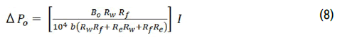

Figure 8. Measured static pressure and characteristics of the mercury DCEMP.
In Eq. (8) since the temperature of the liquid mercury in the performed tests was constant (20°C), the electrical resistances are also constant and so is the magnetic flux density at zero flow, Bo. Based on the results presented in Figure 8b, the determined magnetic flux density in the pump duct (Figure 5) at zero flow of liquid mercury is independent of the values of the electrodes' electrical current and equals 7,750 Gauss.
Wall electrical contact resistance
As indicated in Eqs. (1) and (8), the dynamic and the static pressure for a DC-EMP depend on the electrical resistance of the flowing liquid, Re, the total fringe resistance for the current flows upstream and downstream of the pump duct, Rf, and the electrical resistance of the duct walls, Rw (Figure 3). The calculated values of Re and Rw are functions of the duct and wall dimensions and the electrical resistivities of the liquid and the duct wall materials at 20°C. For mercury DC-EMP of Watt et al. [18], the measured wall resistance, Rw, was 230 μΩ. However, the value determined based on the wall dimensions and electrical resistivity is 217 μΩ. The difference between the measured and calculated wall resistances of 13 μΩ, or 5.65%of the measured value, is because the calculated wall resistance neglects the of wall contact resistance due to brazing or welding. In the absence of the actual measurements, the wall contact resistance is not be possible to quantify.
Figure 9 presents the ECM predictions of the characteristics for mercury DC-EMPs [18] using the measured wall resistance and the calculated values of wall resistance that neglects the contact resistance. Results show when neglecting wall contact resistance, the ECM with input electrical current of 6,740 A overestimates the pumping pressure for the mercury DC-EMPs [18] by 0.64 to 2.346 kPa (0.2 to 1.4%), depending on the mercury flow rate. In these predictions, the ECM used the determined values of the fringe resistance and the magnetic field flux density (Figures 7 and 10) from the reported measurements at zero flow [18].
Magnetic flux density
The reported experimental characteristics of the mercury DC-EMP [18] in Figure 8 are used to determine the dependences of the magnetic flux density, B, on the flow rate of the liquid mercury in the pump duct and input electrical current, I. The values of the magnetic flux density, B, obtained using Eq. (1) from the reported measurements of the net pumping pressure, ΔP, electrodes electrical current, I, and the mercury flow rate, Q, are presented in Figure 8a confirms that the magnetic flux density at zero flow rate, Bo, is independent of the electrodes' current. However, the values of the magnetic flux density, B, decrease with the increased flow rate of liquid mercury and/or the electrical current to the electrodes. The results in Figure 10 show that at mercury flow rate of 15.82 m3/hr, the decrease in B relative to its value at zero-flow value, Bo, varies from 2% to 6.8% with increased electrical current to the electrodes from 10,400 A to 3,970 A, respectively. At an electrical current of 6,740 A, the values of B at mercury flow rates of 15.82 to 26.24 m3/hr are 3.4% and 6.6%lower than Bo. The results in Figure 7b also show that the largest decrease in the magnetic flux density of 7.7% is for electrodes’ current of 5,180 A and mercury flow rate of 22.37 m3/hr. The decreases in the effective magnetic flux density, B, with increased liquid flow rate are due to the corresponding increases of the induced opposing voltage, Ei, due to the flow of the electrically conductive liquid in the applied magnetic field in the pump duct. This induced voltage increases with increased mercury flow (Eq. 7). Therefore, neglecting the effect of the liquid flow rate on the magnetic flux density in the pump duct may result in a few percentages difference between the measured values of the pumping pressures and those predicted using the ECM. The ECM predictions are based on assuming constant values of the magnetic flux density and fringe resistance that equal those for zero flow (i.e.,B=Bo,and Rf = Rfo) (Figure 7).
In summary, the presented results in this section for the mercury DC-EMP designed, constructed, and evaluated by Watt, et al. [18] demonstrate the importance of the reported experimental measurements that included the total electrical resistance and the magnetic flux density at zero flow, the pump static pressure and operation characteristics at different values of the electrical current to the electrodes. These measurements helped determine the values of the total fringe resistance and the effective magnetic flux density with increased electrodes electrical current and flow rate of liquid mercury. Results show the total fringe resistance for the mercury DC-EMP [18] increased with increased mercury flow rate and/or decreased electrodes’ current. The determined total fringe resistance at zero flow=103.782 μΩ and is independent of the input current, while the pump static pressure increases linearly with increased electrical current. For electrical currents from 3,970 A to 10,400 A, the obtained values of the total fringe resistance and the effective magnetic flux density for the mercury pump are 4.3% higher and 7.7% lower, respectively, than their values at zero flow.
Direct measurements of the values and the dependences of the fringe resistance and the magnetic flux density on the liquid flow rate are challenging to perform in practice with acceptable uncertainties. However, the static measurements of the total electrical resistance and the magnetic flux density are much easy to conduct. In the absence of direct experimental measurements for an actual DC-EMP design, it is almost impossible to predict the pump performance a prior with confidence. However, the ECM could calculate the pump performance characteristics subject to the assumptions of constant values of the total fringe resistance and the magnetic flux density, regardless of the liquid flow rate, and neglecting the wall contact resistance. Thus, the ECM analysis needs applicable values of the magnetic flux density and fringe resistance for the pump design concept of interest.
ECM Predictions of the Mercury DC-EMP Characteristics
The next section uses the ECM to predict the performance characteristics of the mercury DC-EMP [18] and compares them to the reported measurements to quantify the effects of the various assumptions on the ECM predictions. Figure 9 compares the ECM predictions of the mercury pump characteristics to the reported experimental measurements for three values of the electrical current values of 3,970 A, 6,740 A, and 10,400 A. The presented predictions are for constant fringe resistance and magnetic flux density values equal to those measured and determined from the reported experimental measurements at zero flow (Rfo and Bo). The predictions of the static pressure at different electrical currents agree with the extension of the reported measurements values. However, the ECM predictions overestimate the measured characteristics of the mercury DC-EMP [18]. with increased liquid flow rate with the difference increasing with increased liquid flow rate and decreased electrodes current to as much as ~6.8% (Figure 10). As the results in this figure show the magnitude of overestimating the pump characteristics using the ECM predictions depends on the values of both the electrical current and the liquid mercury flow rate.
As shown in Figures 9 and 10, assuming constant Rfo and Bo and neglecting their dependences on the input electrical current and the mercury flow rate, and neglecting the pump duct wall contact resistance and the effect of Joule heating on raising the temperatures of the flowing liquid and the pump structure the ECM over predicts the performance characteristics of the mercury DC-EMP. For the same mercury flow rate, the magnitude of overestimating the pumping pressure increases with decreasing the electrical current. For the same electrical current, the magnitude of overestimating the pumping pressure using the ECM also increases with the increasing flow rate of liquid mercury. For example, at a mercury flow rate of 15.82 m3/hr and input currents of 3,970 A, 6.740 A, and 10,400 the ECM overestimates the pumping pressure by 6.85%, 3.38%, and 2.1%, respectively. Similarly, at a mercury flow rate of 26.24 m3/hr. and input currents of 6,740 A and 10,400 A, the ECM overestimates pumping pressure by 6.62% and 3.7%, respectively (Figure 10).

Figure 9. Comparison of ECM predictions of the mercury pump characteristics using measured and calculated wall resistance.

Figure 10. Reported measurements of the magnetic flux density in the pump duct at zero flow and as a function of mercury flow and the input electrical current.
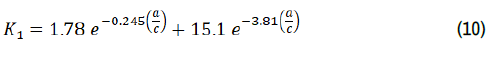
These overestimates are due to the combined effect of the inherent assumptions in the ECM. The actual values of the fringe resistance and the effective magnetic flux density in the pump duct are higher and lower, respectively, than their values at zero flow, which are independent of the input current value. The fringe resistance, however, increases with decreased electrical current and/or increased mercury flow rate. On the other hand, the effective magnetic flux density in the pump duct decreases with decreased electrical current and increased mercury flow rate. Neglecting the duct wall electrical contact resistance decreases the total electrical resistance of the pump duct. The Joule heating would increase the temperatures of the flowing liquid mercury and duct wall and hence their electrical resistance as well as total duct resistance. Suggested empirical expressions the literature used by investigators to estimate the fringe resistance in the ECM analysis. Watt [21] proposed the following expression for calculating fringe resistance in terms of the electrical resistance of the liquid in the pump duct, Re, multiplied by a correction factor, K1, as:

The correction factor, k1, in terms of the ratio of the pump duct width and length (a/c), is:
Baker and Tessier [6] had proposed calculating the fringe resistance from multiplying the effective liquid resistance, Re, with the ratio of pump duct length and width (c/a) and a constant correction factor 2.5, as:

Unlike the results presented in Figure 7 for the mercury pump of Watt et al. [18], the calculated values of Rf using Eqs. (9) and (11) are independent of both the liquid flow rate and the input electrical current. The calculated fringe resistances for the mercury DC-EMP using these expressions are compared in Table 1 to that determined from the reported experimental measurements by Watt et al. [18] at zero flow rate, Rfo=103.782 μΩ.
| Method | Rf  |
difference [%] |
|---|---|---|
| RfoObtained from reported measurements, [18]. | 103.8 | - |
| Rf Calculated using Eq. (9), Watt [21]. | 121.5 | +17.05 |
| Rf Calculated using Eq. (11), Baker and Tessier [6]. | 158 | + 52.2 |
The calculated Rf values using the Watt [21] expression in Eq. (9)=121.5 μΩ, is 17.05% higher than the experimental value. The estimate of Rf using the expression by Baker and Tessier [6] in Eq. (11) is 52.2% higher than the experimental value for zero flow in Figure 7 and Table 1. The values of Rfo in Table 1 are used in the ECM to calculate the characteristics of the mercury pump at an input electrical current of 6,740 A and the measured magnetic flux density at zero flow, Bo=7,750 G. Figure 13 compares the calculated to the experimental characteristics. The high estimates of fringe resistance values using the recommended empirical expressions by Watt [21] and Baker and Tessier [6] increased the ECM predictions of the pumping pressure compared to the reported measurements, which decreased slower with liquid mercury flow rate (Figure 11).

Figure 11. Comparison of ECM predictions of the mercury pump characteristics with reported measurements [18].

Figure 12. The ECM predictions magnitude of overestimating the measured characteristics of the mercury DC-EMP [18].
The ECM predictions of the mercury pumping pressure using Watt's [21] and Baker and Tessier's [6] expression for the fringe resistance are as much as 23.2%, and 15.7% higher than reported measurements [18]. Based on these results, overestimating the fringe resistance and, to a lesser extent, neglecting its dependence on the liquid flow rate (Figure 7a) in ECM results in overestimating the characteristics of the mercury DC-EMP. Instead, with the determined value of the fringe resistance at zero flow, Rfo, from the reported experimental measurements of the pump characteristics and the magnetic flux density at zero flow rate, the ECM overestimated the experimental pump characteristics at electrodes current of 6,740 by only <6.6% (Figure 10). As indicated earlier, this difference could be attributed to not accounting for the dependence of the fringe resistance and the magnetic flux density on the electrodes current and the liquid flow rate (Figure 7), and neglecting the wall contact resistance in the ECM predictions.
Actual experimental measurements for an existing pump design [18], could quantify the effects of the assumptions in the ECM on the predictions of the pump performance. In the absence of such measurements using the ECM to estimate the performance of a DC-EMP for meeting certain performance requirements is easy, but predictions of the pump characteristics will be higher than actual. The present results have shown that such over prediction is due to the inherent assumptions in the ECM such as using constant values of the fringe resistance and the magnetic flux density that equal those at zero flow, Rfo and Bo, respectively. Nonetheless, the ECM results would be useful for optimizing the design prior to the fabrication of the pump. Therefore, for given magnet and pump designs and working fluid, there is a need to accurately calculate the values Rfo and Bo to incorporate in the ECM for calculating the pump characteristics and performing parametric analysis to optimize the pump design, which is a focus of the present work described in the following section.
Finite Element Method Magnetics (FEMM) software
This section is to demonstrate the effectiveness and accuracy of the FEMM software for calculating the fringe resistance and the magnetic flux density at zero flow, Rfo, and Bo, respectively. To estimate Bo, however, the FEMM software requires the actual magnet dimensions. However, Watt et al. [18] did not provide these dimensions for the mercury pump. The accuracy of FEMM software for calculating Bo is determined by comparing its predictions to reported measurements for different magnet designs with stagnant liquids. The FEMM is open-source software for solving magneto static problems, magnet time-harmonic, electrostatic, electric current flow, and steady-state heat flow in two-dimensional planar and axisymmetric domains [28]. The input CAD-geometry of the magnet and computational domain are discretized into a triangular first-order grid of finite mesh elements. The software includes traditional variation formulation for solving relevant partial differential equations and built-in libraries of physical thermal, electrical and magnetic properties of varied materials. Users may predefine the largest mesh element sizes in the numerical grid in the different regions of the computation domain or use the built-in mesh auto-generator. The software allows inspecting the fields’ solutions at arbitrary points or contours of the geometry for exporting or plotting various parameters of interest [29].
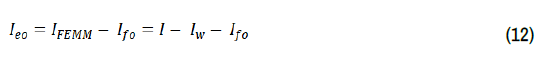
Linking the FEMM inter-process communications to MATLAB [29] significantly reduces the processing time and that for extracting and graphically displaying and plotting the results. This linking is quite effective for performing a DC-EMP design optimization that requires a substantial number of FEMM simulations to calculate the values of the fringe resistance and magnetic flux density at zero flow, Rfo, and Bo, respectively. These values are used in the ECM to calculate the performance different pump designs. The entire process is fast and effective for down selecting a pump design before the actual fabrication and assembly of the pump components. As shown in Figure 7a, the values of Rfo for the mercury pump are independent of the input electrical current. The specified effective electrical current in the FEMM analysis, IFEMM, equals the input current, I, minus the wall current, IW, thus IFEMM=I – IW. In addition, the user specifies the materials of choice for the pump duct wall, current electrodes, the working fluid, and the total input electrical current to the electrode for a zero-voltage at the surface of the exit current electrode. The FEMM software then calculates the current density distribution including the total fringe current, Ifo, flowing through the liquid upstream and downstream of the pump duct. The calculated Ifo value when subtracted from the input electrical current to the FEMM software, IFEMM, gives the effect current across the static liquid in the pump duct, Ieo, as:
The present work calculated the fringe resistance in terms of the effective electrical current, Ieo, and the electrical resistance of the static liquid in the duct, Re, as:
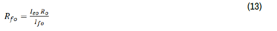
The calculated value of Re in Eq. (13) is based on the dimensions of
the pump duct and the electric resistivity of the working fluid,  , at the
liquid temperature, as
, at the
liquid temperature, as

The FEMM calculates the magnetic flux density at zero flow using the Magnetics package, which simulates both permeant and induced magnets. It solves Maxwell’s equations of Gauss's law for magnetism and Ampere’s law [29] for the planner distribution of the magnetic flux density, Bo(y, z), in the pump duct at zero flow (Figure 7). In these calculations, the FEMM material libraries provide the magnetic permeability, B-H curves, and magnetization directions of permanent magnets. The following equation calculated the effective magnetic flux density in the pump duct at zero liquid flow, Bo, [29], as:
FEMM analyses
In this section, analysis of the current flow field in the mercury DC-EMP [18] is conducted to calculate the fringe resistance at zero flow rate, Rfo, using the FEMM software and compare it to that obtained from the reported electrical measurements (Figure 7a). Because the magnet dimensions were not reported for the mercury DC-EMP by Watt et al. [18], it was not possible to conduct FEMM analysis to determine the value of the magnetic flux density at zero flow, Bo, and compare it to the values obtained from the reported experimental measurements. Therefore, to validate the FEMM capability of calculating Bo, this work conducted field analysis of the seawater thruster reported by Li et al [29] using the FEMM software and the calculated values of the magnetic flux density at zero flow, Bo, are compared to reported measurements [29]. The results presented in Figure 7 For the mercury DC-EMP shows that Rfo and Bo is independent of the value of the current electrode. The following subsections detail the performed FEMM analysis for calculating both Rfo and Bo.
Fringe resistance at zero flow
The input to the performed FEMM analyses to calculate the fringe resistance at
zero flow of mercury, Rfo, for the mercury DC-EMP of Watt et al. [18], includes
the pump duct dimensions and materials. To provide details of the fringe current
density field lines, the used lengths of the downstream and upstream sections of
the pump duct in the FEMM calculations are longer than half the pump duct
length, c (Figure 13). The FEMM built-in auto mesh generator produced the
numerical meshing of the computation domain. The used electrode electrical
current in the performed analysis, IFEMM=6,155 A. Figure 15 presents the
calculated current density, ![]() , field distribution in the pump duct. The current
density distributions are symmetric in the left and right halves and in the top and
bottom halves of the pump duct. At the mid-plane of the pump duct, the current
density is ~0.9 A/mm2, which is less than the input current density of 1.12 A/
mm2. Four regions in the pump duct near the edges of the current electrodes
indicate large current densities ~1.4 A/mm2. This edge effect is caused by the
movement of electrons toward regions of high geometric gradients (Figure 13).
The results also show a gradual decrease in current density with increased
distance along the z-axis until eventually reaching zero (Figure 13). The
computation domain extending from the input and the exit of the pump duct
shows the fringe currents (Figures 13 and 14) flow paths in the top half of the
pump duct and the downstream section of the duct. The flow lines of the
electrical current across the pump duct are mostly uniform but experience a
curvature when exiting the pump duct into the upstream and downstream
regions (Figure 14).
, field distribution in the pump duct. The current
density distributions are symmetric in the left and right halves and in the top and
bottom halves of the pump duct. At the mid-plane of the pump duct, the current
density is ~0.9 A/mm2, which is less than the input current density of 1.12 A/
mm2. Four regions in the pump duct near the edges of the current electrodes
indicate large current densities ~1.4 A/mm2. This edge effect is caused by the
movement of electrons toward regions of high geometric gradients (Figure 13).
The results also show a gradual decrease in current density with increased
distance along the z-axis until eventually reaching zero (Figure 13). The
computation domain extending from the input and the exit of the pump duct
shows the fringe currents (Figures 13 and 14) flow paths in the top half of the
pump duct and the downstream section of the duct. The flow lines of the
electrical current across the pump duct are mostly uniform but experience a
curvature when exiting the pump duct into the upstream and downstream
regions (Figure 14).

Figure 13. Comparison of the experimental characteristics of the mercury Pump to those calculated using ECM with different values of Rfo and input electrical current of 6740A.

Figure 14. Calculated 2-D magnetic flux density field, Bo (y, z) by FEMM software [29].

Figure 15. The calculated electrical current flow field in the duct and the upstream and downstream sections of the mercury DC-EMP at zero flow using the FEMM software.
Integrating the calculated current flow fields in the pump duct and both upstream and downstream of the duct determines the effective current flow across the duct, leo, and the total fringe current, lfo, respectively. The solutions of Eqs. (13) and (14) determine the total fringe resistance, Rfo, using the calculated fringe current and the current flow in the duct. The calculated total fringe resistance for the mercury DC-EMP using a largest numerical mesh element size of 0.2 mm in the FEMM analysis is 104.59 μΩ, which is only ~0.8% higher than the value of 103.78 μΩ obtained from the reported experimental measurement (Figure 7a) (Table 2). This excellent agreement demonstrates the effectiveness and accuracy of the FEMM analysis for calculating the fringe resistance in DC-EMPs at zero flow. The next subsection presents the results of investigating the effect of changing the numerical mesh element size in the computation domain in the FEMM analyses on the calculated values of the total fringe resistance, Rfo, for the mercury DC-EMP [18].
| Parameter | Largest mesh element size (mm) | ||
|---|---|---|---|
| ~ 2.0* | 0.5 | 0.25 | |
| Calculated fringe resistance,Rfo (μΩ) | 104.58 | 104.50 | 104.48 |
| Total number of mesh elements | 46,650 | 538,861 | 2,108,441 |
| normalized value | 1.0 | 11.55 | 45.2 |
| Computation real time (s)** | 4.5 | 47.75 | 187.25 |
| Normalized value | 1.0 | 10.6 | 41.6 |
"Mesh auto-generator"; **Using Intel octa-core i7-8665U CPU @ 2.1 GHz
Sensitivity analysis
Figure 15 presents examples of the applied numerical mesh grid within the computation domain in portions of the pump duct and the upstream section of the duct. The size of the numerical mesh elements in the liquid region is largest at the center of the duct and decreases gradually with decreasing distance from the interface between the liquid and the inner surface of the duct wall. Near this interface, the size of the numerical mesh elements in the liquid is the smallest. Similarly, the size of the numerical grid mesh elements in the current electrode and the surrounding air within the computation domain (Figures 16 and 17) is smallest near the interface with the outer surface of the duct wall. The mesh auto-generator in the FEMM software generated the numerical mesh grid within the computation domain (Figure 15) with the largest mesh element size of ~2.0 mm in the ambient air region. Additional analyses are performed with finer numerical mesh grids with smaller sizes of 0.25 and 0.5 mm of the largest mesh elements to quantify the effect of numerical mesh refinements on the calculated values of Rfo for the mercury DC-EMP [18].

Figure 16. The calculated electrical current flow field in the duct of the mercury DC-EMP [18].

Figure 17. An example of applied numerical mesh grid with largest mesh element size of ~ 2.0 mm in the FEMM software to calculate Rfo for the mercury DC-EMP with (Table 2).
Table 2 compares the results of the performed analysis of calculating Rfo for the mercury DC-EMP [18], using the FEMM software with coarse and fine numerical mesh grids. Results show that increasing the refinement of the applied numerical mesh grid negligibly changes the calculated value of Rfo<0.1% but significantly increases the total number of the numerical mesh elements in the computation domain and the computation time using the same hardware. The numerical mesh refinement with the computation domain decreases the size of the largest mesh element in the applied numerical grid in the FEMM analysis from ~2 mm to 0.5 and 0.25 mm. Therefore, a numerical mesh grid produced by the FEMM mesh auto-generator with the largest mesh element size of ~2 mm is a practical choice considering the large savings in the computation time without impacting the results.
It is worth noting that the calculated value of Rfo using the present FEMM analysis of 104.48 μΩ is only 0.56% higher than that obtained from the report experimental measurements (103.8 μΩ) for the mercury DC-EMP by Watt et al. (1957) (Table 2). In comparison, the suggested correlations of Watt [21], Eq (9) and (10), and Baker and Tessier [6], Eq. (11), overpredict the value of Rfo by 17% and 52%, respectively (Table 1). Consequently, the calculated characteristics of the mercury DC-EMP [18] using the ECM with the Rfo values based on the proposed expressions by Watt's [21] and Baker and Tessier's [6] are as much as 23.2% and 15.7% higher, respectively, than the reported measurements [18] (Figure 11).
The next subsection examines the accuracy of the FEMM software analysis for predicting the magnetic flux density at zero flow, Bo. It was not possible to calculate Bo for the mercury DC-EMP because Watt et al. [18] did not report the needed magnet dimensions in the input to the FEMM analyses. Instead, the present work compared the calculated Bo value using FEMM analysis for a permanent magnet in an MHD thruster for seawater propulsion (Figure 18) to the reported experimental value [30].

Figure 18. Isometric view of the MHD thruster of Li et al. [30].
Magnetic flux density at zero flow
The operation principle of an MHD thruster is like that of a DC-EMP. In the latter, the
induced Lorenz force drives the liquid in the pump duct, while in the former this force moves the thruster relative to the liquid. The MHD thruster reported by Li et al. [30] employs NdFeB (N35) permanent magnets, Aluminum electrodes, plastic electrical insulation, metal housing, and saltwater working fluid (Figure 16). The total length of the thruster is 100 mm, the square liquid flow region is 50 mm on the side, and the magnet is 10 mm thick. Li et al. [30] measured the magnetic flux density along the y-axis at the mid-plane of the thruster liquid region (x = 0, z = 0) with the metal shell removed. Figure 19 presents the reported measurements of the magnetic flux density along the yaxis. They are highest in the middle of the duct (y=20 mm) and decrease rapidly with increased distance toward the two ends of the thruster. The measured values of the magnetic flux density are symmetric except near the ends of the thruster. The slight asymmetry may be due to imperfections in the manufacturing of the magnets.

Figure 19. Comparison of the axial distribution of the measured values of the magnetic flux density for an MHD thruster [30] at zero flow to that calculated using FEMM analysis.
The present analysis compared the calculated values of the magnetic flux
density along the y-axis of the thruster duct using the FEMM software to the
reported measurements in Figure 17 [30]. There is excellent agreement between the calculated and measured values of the magnetic flux density,
across the thruster duct, except near the ends of the magnet where the
calculated values are slightly lower than the reported measurements by
Li et al. [30], These differences, however, insignificantly affect the
value of the average magnetic flux density, , based on the calculated
lateral distribution of the local values in the thruster duct region. The
determined value of , based on the reported measurements of the axial
distribution of the magnetic flux density in Figure 17 is ~9.955 × 10² T,
compared to 9.962 × 10² T for the calculated value based on the FEMM
analysis results, a difference of less than 0.1%. These results confirm the
accuracy of the FEMM analysis for calculating the magnetic flux density
for permanent magnets at zero flow.
, based on the calculated
lateral distribution of the local values in the thruster duct region. The
determined value of , based on the reported measurements of the axial
distribution of the magnetic flux density in Figure 17 is ~9.955 × 10² T,
compared to 9.962 × 10² T for the calculated value based on the FEMM
analysis results, a difference of less than 0.1%. These results confirm the
accuracy of the FEMM analysis for calculating the magnetic flux density
for permanent magnets at zero flow.
The analysis of the reported experimental measurements for the mercury DC-EMP determined the values of the total fringe resistance, Rf, and the magnetic flux density, B, in the pump duct and their dependence on the electrodes’ electrical current and the flow rate of mercury at 20°C. Results show that Rf increases with decreased electrical current and increased flow rate of liquid mercury, while the magnetic flux density decreases with increased flow rate and decreased electrical current. Results also show that the pumping pressure decreases with increased flow rate of mercury and/or decreased electrical current. The pump static pressure at zero flow increases linearly with increased electrical current While the values of the fringe resistance and the magnetic flux density at zero flow, Rfo, and Bo, respectively, are independent of the value of the electrical current. The present ECM analysis uses these values and that of the measured wall contact resistance to predict the pump characteristics and compare them to the reported measurements.
The present work investigated using the current flow package of the 2-D FEMM software for calculating Rfo for the Mercury DC-EMP. The calculated value is in excellent agreement with that from the reported measurement to within 0.8%. The present analysis used the FEMM magnetic package to calculateBo, of NdFeB (N35) permanent magnet for an MHD thruster. The average value of 9.962 × 10² T calculated using the FEMM software is within only 0.1% of that measured, ~9.955 × 10² T. These results confirm the accuracy of the FEMM software for calculating Rfo and Bo for DCEMPs. Incorporating the values for the mercury DC-EMP into the ECM analysis, the predicted characteristics at different electrical current values are consistently higher than the reported measurements by <10%, depending on the value of the electrical current. These ECM results show that neglecting the measure wall electrical contact resistance of 13 μΩ decreases the ECM predictions of the pump characteristics by ~0.2%-1.4%, depending on the liquid mercury flow rate.
Therefore, the ECM may be used to perform parametric analysis and predict the performance of DC-EMP designs prior to construction using the calculated values of Rfo and Bo by the FEMM software, based on the selected dimensions of the liquid flow duct, electrical current electrodes, and the magnet. However, although are consistent with those of the actual pumps after construction, the ECM predictions can overestimate the pump characteristics but by ~<10%. This is due neglecting the effects of the liquid flow and the electrical current on the fringe resistance and the magnetic flux density in the pump duct, and the electrical contact resistance of the duct wall.
The University of New Mexico’s Institute for Space and Nuclear Power Studies funded this research.
[Crossref] [Google Scholar] [PubMed]
Journal of Material Sciences & Engineering received 3677 citations as per Google Scholar report