Estimation of Some Thermal Diffusion Parameters by Coupling the Fractional Derivative Theory and the Genetic Algorithm

Rasolomampiandry G^1*, Rakotoson R² and Randimbindrainibe F^3
*Correspondence: Rasolomampiandry G, Cognitive Sciences and Applications Research Laboratory, BP 1500, Ankatso - Antananarivo 101, Madagascar, Email:

Keywords

Genetic algorithm • Thermisorel

Introduction

In [1], a heat transfer study was performed on a sample of low density wood fiber board, called Thermisorel. This material is manufactured by STEICO Casteljaloux in France. Thermisorel is used in construction because it prevents heat loss in winter due to their low thermal conductivity, nearly 0.042 Wm-1 K-1. It also protects the building from heat in summer due to their capacity high thermal storage. In this study, a 22.2 mm thick thermisorel board was used. The details of this study are described [1]. Only the data necessary for our problem mentioned above, which we will recall. This work will be divided into two parts:

In section 2, we will detail the position of our problem, as well as the hypotheses necessary for its resolution. In the third part, we will talk about the genetic algorithm, as well as the time fractional diffusion equation and its discretization in order to give the desired solution

Positioning of the problem

Our problem is to identify suitable optimal values of thermal conductivity and thickness of a thermal insulator, if we vary from 15°C to 24.6°C the temperature of one of the faces and the other will keep a constant temperature of 15°. To solve this problem, we will use as hypotheses, the data used from the experiment in [1]:

- The density of the insulation: ρ =170kg.m⁻³

- Specific heat: C_p =1280 J kg K⁻¹ (according to the measurement made by the CSBT)

- Temperature and heat flux variations as a function of time, on both sides of the thermal insulator plate (see tables below)

From the graphs in [1], we extracted the values of the temperature and those of the flux as a function of time, until the steady state was reached, for the hot side. We have the following tables (Tables 1-3):

Additional assumptions are introduced:

- Since the temperature and the heat flux at any point of each face, at a given time, are identical, then we can restrict the study to a straight segment perpendicular to the two faces, one of the ends of which (noted O) on hot face and the other (noted X) on the face where the temperature is constant

- It is assumed that the variation of the flux, at a given moment, on this segment is linear

The problem thus turns to the following question:

What are the optimal values suitable for thermal conductivity and segment length [O, X]? If the temperature at point O varies according to Table 1,2&3 during the transient period. And that the temperature of the X end is 15°C during the two regimes, permanent and stationary.

The solution is therefore the values of these two parameters which can give at point X the temperature value closest to 15°C. (If we use the means mentioned at the beginning)

Solution of the Problem by Coupling the Genetic Algorithm and the Fractional Diffusion Equation

The time fractional diffusion equation

In the case of this problem the time fractional diffusion equation is written:

Caputo of order α, 0 <α <1 of the variable t, t> 0 [2,3]

be determined and which corresponds to the thickness of the thermal insulator

is the diffusivity coefficient. kis the other parameter to be determined

T(t, x) is the temperature corresponding to the variables t and x

f (t, x) is the flow corresponding to the variables t and x

For our discretization:

Note that the transient regime stops at the 130th second. Then on the segment [0,T₀ ]

And [0, X ] , we respectively construct a finite sequence such that

and t_i = il , a finite sequence that and x_j = j_h

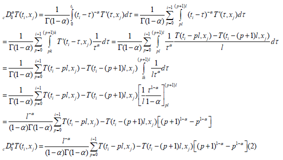
This relation is valid for i ≠ 0

For the Laplacian discretization we will use the advanced decentered differentiation [4] and we have:

                  (3)

The linearity assumption on f (t, x) allows us to write:

Equation (1) has become:

To simplify the writing, note hence

and the équation (5) has become:

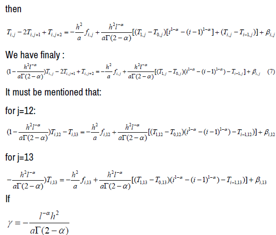
We further assume that for

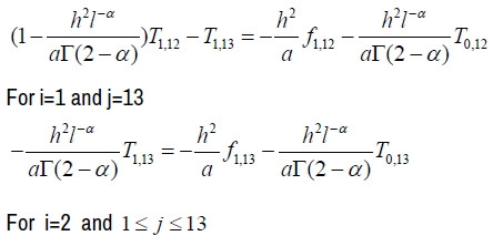
For i =1 et 1≤ j ≤13 , (5) is written:

Specifically

For i = 1 and j = 12 we have

We deduce the following matrix forms:

For i =1;1≤ j ≤13

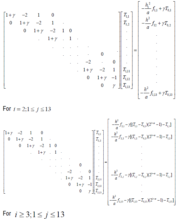
We then have 13 matrix equations of the form

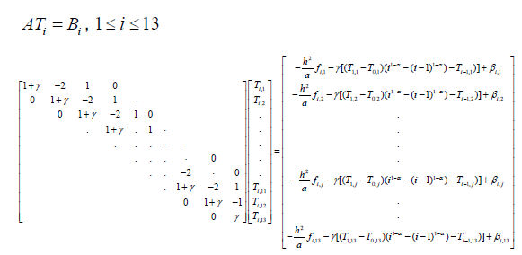
If we fix kc and X, the solution of these equations following the values of i , gives

us a value of T(13,13) , when i=13 and which the value of the temperature

at the point X . If T(13,13) =15°C then k_c and X are the solutions of the problem posed. Otherwise we change the value of k_c and X. We only stop if T(13,13) =15°C

To speed up the search of k_c and X, we set the search intervals for the two parameters and by means of the genetic algorithm, we can give optimal values, which depends on the imposed acceptance

The genetic algorithm

For the classical method, to identify a parameter θ , suitable for a given problem, in a set A, we consider a finite sequence of elements of A and among these elements we look for what respects the imposed conditions. If none of these elements is valid, we change immediately until we have an optimal solution. This process is long and can lead to a lot of wasted time in some cases [5].

Regarding the genetic algorithm, the choice of θ is made directly in A, even if A is uncountable; everything is predefined to avoid wasting time

Optimal values of X and K _C

If α = 0.9 is the order of the fractional derivative. If we choose [0.03;0.045] c k ∈ and X ∈[0.02;0.03] , the computation with MATLAB, by means of the genetic algorithm, gives us the optimal solution:

. There is a difference between the values pronounced during the experiment and the values found by means of the genetic algorithm. But if we use as a hypothesis these theoretical values in [6] for example, we arrive at the same result.

Conclusion

In this article, we made an example of the coupling of a fractional differential equation and the genetic algorithm to optimize certain physical parameters. In future publications we will consider yet another fractional differential equation suitable for another physical system and which we will couple with an algorithm, such as what we used to optimize certain parameters.

References

1. Kaemmerlen A, Asllanaj F,  Sallée H, Baillis D and Jeandel G. ‘‘Transient modeling of combined conduction and radiation in Wood fibreinsulation and comparison with experimental data’’. Int. J. Therm. Sci 49 (2010) :2169-2176
2. Kilbas Anatoly, Srivatastava Hari M and  Trujilio Juan J. ‘‘Theory and applications of fractional differential équations.’’  204 (2006) : 1-523
3. Podlubny Igor. ‘’Fractional Differential équations.’’ Academic Press (1998) : 340
4. Buffat Pr Marc‘Approximation of derivatives by finite differences.’’
5. Yang Q, Liu F and Turner I. ‘’Numericals methods for fractionnal partial differential equations with Riesz space fractionnal derivatives.’’ Appl. Math. Model.34(2010) : 200-218
6. Yang Won Y, Cao Wenwu, Chung Tae-Sang and   Morriset John .Applied Numerical Methods Using Matlab. DOI:10.1002/0471705195. (2005