Research Article - (2024) Volume 15, Issue 2
Received: 11-Mar-2024, Manuscript No. jbmbs-24-129172;
Editor assigned: 13-Mar-2024, Pre QC No. P-129172;
Reviewed: 27-Mar-2024, QC No. Q-129172;
Revised: 01-Apr-2024, Manuscript No. R-129172;
Published:
08-Apr-2024
, DOI: 10.37421/2155-6180.2024.15.212
Citation: Li, Fengnan and Shein Chung Chow. “Evaluating
Reproducibility and Generalizability of a Medical Predictive Model in Clinical
Research.” J Biom Biosta 15 (2024): 212.
Copyright: © 2024 Li F, et al. This is an open-access article distributed under the terms of the Creative Commons Attribution License, which permits unrestricted use, distribution, and reproduction in any medium, provided the original author and source are credited.
In clinical research, a medical predictive model is intended to provide insight into the impact of risk factors (predictors) such as demographics and patient characteristics on clinical outcomes. A validated medical predictive model informs disease status and treatment effects under study. More importantly, it can be used for disease management. However, a gap in the development process of these models is often observed. That is, most studies only focus on the internal validation for the model's reproducibility but overlook the external validation needed for evaluating generalizability. To solve this issue, this article proposes several methods for assessing both the reproducibility and generalizability of a developed/ validated medical predictive model. The generalizability estimation approaches allow for sensitivity analysis in situations where data on new populations is not available, which provides valuable insights into the model's applicability to patients from a different population.
Internal validation • Reproducibility • External validation • Generalizability
Medical predictive models have long played a crucial role in clinical research and practice, especially in recent times when personalized medicine has become increasingly popular. Usually, a medical predictive model is designed to express a clinical outcome (response) as a function of a multivariate set of predictors (risk factors). It offers valuable insight into the association between clinical outcomes and predictors and more importantly, facilitates disease management. Such models can be either diagnostic or prognostic. A diagnostic model reflects the patient's current health conditions, while a prognostic model estimates the probability or risk of developing an outcome over a specific period. For example, the Framingham Risk Score is a prognostic medical predictive model that takes a multivariate set of risk factors as input and estimates the 10-year risk of developing cardiovascular disease [1].
The procedure for developing a medical predictive model involves the following steps:
(i) Predictor Identification, where potential predictors are identified and a subset to be included in the model is selected via regression methods.
(ii) Collinearity testing, which involves detecting and addressing collinearity among predictors to enhance the model's parsimony and interpretability.
(iii) Model Building, which estimates the coefficients by fitting a regression model based on the identified predictors and assesses the goodness-of-fit.
(iv) Model Validation, comprising interval validation for reproducibility and external validation for generalizability.
Among the four critical steps discussed above, the current issue often arises from the phase of model validation. Internal validation for reproducibility refers to the model's ability to replicate the results when applied to new data from the same population (e.g., data collected from the same medical center). External validation for generalizability refers to the extent to which the predictive model is applicable across different populations (e.g., different age groups or ethnic groups). Ideally, a comprehensive validation of a medical predictive model should include both internal and external validations. However, in practice, we find that most of the model's development only performs the internal validation. The process of external validation to assess the model's generalizability is often hindered by the unavailability or the prohibitive cost of acquiring the new population's data. In response to the issue in the model's validation, we propose several methods for estimating both the reproducibility and generalizability probability of a medical predictive model. The approaches for generalizability assessment are developed by adapting the reproducibility probability estimation methods, which effectively estimate the model’s generalizability to new populations.
The remaining parts of the paper are organized as follows. In below section summarizes the procedure for developing a medical predictive model and discusses the critical issue regarding the model's validation. In the below section addresses this issue by proposing methods for reproducibility and generalizability assessment. Concluding remarks are given in the last section of this article.
Predictive model building and validation
Procedure for model development: Usually, the procedure for developing a medical predictive model in practice involves the following four steps: predictor identification, collinearity testing, model building, and model validation, which are discussed in detail as follows.
Predictor identification: The foundational step in building a medical predictive model is to identify the predictors (risk factors) to be included in the model. Potential predictors are obtained from demographics and patient characteristics information at baseline. To ascertain the relationship between a predictor and the clinical outcome, the Pearson correlation coefficient can be applied as a measure of correlation. A commonly used rule of thumb is that a correlation coefficient greater than 0.3 indicates a moderate correlation and we can consider including the predictor in the model. After collecting the set of correlated predictors, we need to further assess whether the inclusion of a predictor can improve the model's predictive ability. A subset of all the correlated predictors is obtained by sequential selection methods like forward, backward, or stepwise selection, which forms the final set of predictors in the model.
Collinearity testing: Particular attention should be paid to the collinearity among predictors. Even though the collinearity issue does not affect the overall predictive power of the model, it seriously impedes the model's interpretability by inflating the coefficient and confounding the corresponding t-statistics [2,3]. Also, the correlated predictors add unnecessary complexity to the model. By removing or combining these predictors, we can reduce the number of predictors in the model and thus improve the model's performance in fitting new, unseen data.
In addition to the correlation coefficient that measures the collinearity between two predictors, the Variance Inflation Factor (VIF) is applied to quantify the correlation between one predictor and the collective of other predictors in the model. Furthermore, the Condition Number (CN) provides a measure of the overall multicollinearity level within the model [4]. Once a high level of collinearity within the predictors is detected, various techniques can be employed to address the collinearity. We suggest the use of a composite index approach proposed by Chow SC, et al. [5]. This method develops a composite index via ordinary least squares regression to combine multiple correlated predictors into a single predictor. This approach stands out among other collinearity resolution techniques like PCA because it accounts for the outcome variable and preserves the predictors’ correlation with the outcome.
Model building: Previous steps yield the final set of predictors, with the collinearity issue being addressed. Statistical models utilized to build a medical predictive model are usually generalized linear models. A linear regression model is chosen for continuous clinical outcomes. Logistic regression is often utilized for binary outcomes. For time-to-event outcomes, Cox regression is applied. After fitting the data upon a specified model, the goodness-of-fit needs to be measured. For continuous outcomes, R2 or adjusted R2 is commonly applied to evaluate the model's performance in fitting the data. For categorical clinical outcomes, the evaluation of the model's performance involves two aspects: discrimination and calibration. Discrimination measures how well the model distinguishes between different outcome categories and calibration assesses how well the predicted probabilities match the observed frequencies.
Model validation: The final step is model validation which involves internal validation for reproducibility and external validation for generalizability. Reproducibility denotes the ability to replicate the results when the model is applied to new data from the same population (e.g., data collected from the same medical center). In contrast, generalizability refers to the extent to which the model's predictions are applicable across various populations [6].
Critical issue in model development: A critical issue in the predictive model development process is the absence of external validation. After a model is validated in one population, it is often of interest to evaluate whether the model is applicable across different populations (e.g., different age groups or different ethnic groups). Although researchers always aspire to broaden the model's applicability and theoretically an external validation should be performed to evaluate the model's generalizability, in practice, we find that most of the predictive model development efforts halt at the phase of internal validation. This premature termination in model development is often due to the unavailability or the prohibitive cost of acquiring the new population's data. To solve this issue, we first propose three methods for estimating the reproducibility probability of a predictive model. Subsequently, we adapt these reproducibility methods to enable the assessment of generalizability, which serves as a substitute sensitivity analysis when the data of other populations are not present. More details about the proposed methods are discussed in below section.
Statistical methods for assessing reproducibility and generalizability
Internal validation for reproducibility assesses whether results from one study are reproducible in another study where data are collected from the same population, whereas external validation for generalizability evaluates whether the model is applicable across various populations. We find most of the validation process for medical predictive models in practice focuses solely on the internal validation within the same medical centre and the external validation for generalizability is missing. This section aims to resolve this issue by proposing three approaches to estimating the model's generalizability probability. The organization of this section is as follows: In first, section estimation of reproducibility probability proposes three approaches to estimating the model's reproducibility probability. Building upon these reproducibility estimation methods, In second, section estimation of generalizability probability adjusts the approaches in section estimation of reproducibility probability to allow for generalizability probability estimation. The reproducibility or generalizability probability can be defined by either the relative difference or the absolute difference between the true clinical outcome and the predicted clinical outcome. That is,
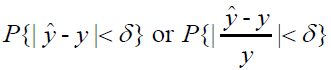
Where �� is pre-determined, clinically negligible value. The following
sections use  as the reproducibility probability as
  follows
a normal distribution, which yields more analytical results. Moreover, the
methods proposed are in the context of a linear re gression model, where a
closed-form solution for coefficients is utilized to estimate the probability.
follows
a normal distribution, which yields more analytical results. Moreover, the
methods proposed are in the context of a linear re gression model, where a
closed-form solution for coefficients is utilized to estimate the probability.
Estimation of reproducibility probability
This section provides three approaches to estimating reproducibility probability, which aims to establish a foundation for the generalizability estimation methods proposed in this section Shao J and Chow SC, et al. [7] proposed three methods for estimating reproducibility probability in clinical trials, the estimated power approach, the confidence bound approach, and the Bayesian approach, to assess the probability of replicating results of the first clinical trial in a subsequent trial with the same study protocol. The key ideas are as follows: the estimated power approach directly replaces the model's parameter in the second trial with its estimate obtained from the first trial; the confidence bound approach accounts for the variation in the estimated parameter and thus uses a lower confidence bound for more conservative estimation and the Bayesian approach calculates the reproducibility probability as a posterior mean. Although the methodologies in medical predictive models and clinical trials are completely different, these ideas can be referred to when estimating the reproducibility probability for predictive models by analogizing the model-building process to the first clinical trial and the validation phase to the second clinical trial.
Approach 1: Similar to the estimated power approach proposed in Shao,
et al.'s paper, approach 1 substitutes the estimated regression coefficients  for the true regression coefficients β. Given an observation
  in the
validation dataset, we have
in the
validation dataset, we have
 (1)
(1)
Where  and p is the number of parameters in the model
The estimated response
and p is the number of parameters in the model
The estimated response  equals
  . we replace β by the estimated in Eq. (1), the difference between the estimated response value
  and observed response value y* would solely result from the error term
coefficient
and observed response value y* would solely result from the error term
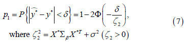
coefficient  . Then the reproducibility probability p1 is:
 (2)
(2)
σ2 can be estimated by  where
where  is the ith data
point in the training set that has n observations in total.
is the ith data
point in the training set that has n observations in total.
p1 estimates the reproducibility probability for a given observation. Utilizing p1, the overall reproducibility of the validation dataset can be evaluated.
Assuming the validation dataset has n observations, the count of reproducible
observations follows a Binomial distribution 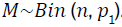 For large sample
sizes, this approximates a normal distribution
For large sample
sizes, this approximates a normal distribution 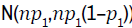 . For instance,
to estimate the probability that at least 95% of the data points are reproducible,
we use
. For instance,
to estimate the probability that at least 95% of the data points are reproducible,
we use

where Φ denotes the cumulative distribution function of the standard normal distribution.
Approach 2: The reproducibility probability estimated by approach 1
is rather optimistic, especially when the variance of is large. In contrast,
approach 2 accounts for the variation of the estimated coefficient rather than
directly substitute it for the true parameter.
The notations are as follows: in the dataset used for model building, we
have Y = Xβ+ ∈, where  represents the response vector,
  is
the design matrix for predictors,
is
the design matrix for predictors,  is the coefficient vector, and
  is
the error term with each element ∈i following a normal distribution N (0,σ2). In
the validation dataset, for a new observation (X*,y*), The model is
is
the error term with each element ∈i following a normal distribution N (0,σ2). In
the validation dataset, for a new observation (X*,y*), The model is
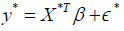
Where 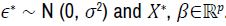 The estimated coefficient vector is
  . The same notations will be used throughout this section. is an unbiased estimator, the expected value of
  is 0. The variance of
the residual is given by
is 0. The variance of
the residual is given by

Since both  and y* are normally distributed, we have
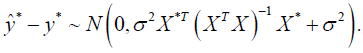
Therefore, for approach 2, the reproducibility probability for an observation (X*,y*) is

Approach 3 (Bayesian approach): Approach 3 utilizes Bayesian inference and prediction for reproducibility probability allows us to estimate calculation, which the uncertainty in the regression coefficients β.
Denote data points in the training set as D and assume σ2, the variance of the error term ∈, is known already. From the Bayesian perspective, the posterior distribution π (β|D, σ) is expressed as

The likelihood  is normal and
  . The
posterior distribution will be normal if a conjugate normal prior is specified.
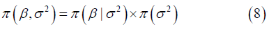
Suppose our choice for the prior is
. The
posterior distribution will be normal if a conjugate normal prior is specified.
Suppose our choice for the prior is 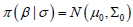 . The posterior distribution
  can be derived subsequently, which is given in the form of

Similarly, if we choose a non-informative prior of  the posterior
distribution will be
the posterior
distribution will be 
Based on the posterior distribution  the posterior predictive
distribution for a new observation (X*,y*) in the validation dataset can be
derived. Given
the posterior predictive
distribution for a new observation (X*,y*) in the validation dataset can be
derived. Given  the
posterior predictive distribution
the
posterior predictive distribution  is then expressed as

Our estimation  for the response value
  is the mean of posterior
predictive distribution, which is
is the mean of posterior
predictive distribution, which is  Consequently, the distribution of
  should be
  . And the reproducibility probability p1 is
given by
. And the reproducibility probability p1 is
given by
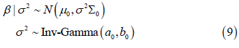
For a more realistic case in practice where σ2 is unknown, we need to specify a prior for the error term variance. Now the prior distribution is
A conjugate prior that leads to an analytical posterior distribution would be the Normal-Inverse-Gamma distribution, where
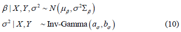
Given the conjugate prior, the posterior distribution 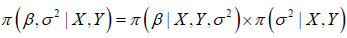 can be derived. The result is
expressed as
can be derived. The result is
expressed as

Subsequently, for a new observation  , the posterior predictive
distribution
, the posterior predictive
distribution  is
is

Integrating both the uncertainty in β and σ2, the posterior predictive distribution would follow a Student's t distribution, which is given by

where  is the location parameter and
  is the
scale parameter. We take
is the
scale parameter. We take  the mean of the posterior distribution
as our prediction for y*. The difference
the mean of the posterior distribution
as our prediction for y*. The difference  would follow a t-distribution
of
would follow a t-distribution
of 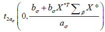 . The reproducibility probability can be
subsequently estimated by transforming the random variable into a standard
t-distribution, which is expressed as
. The reproducibility probability can be
subsequently estimated by transforming the random variable into a standard
t-distribution, which is expressed as

 denotes the cumulative distribution function of a standard
t-distribution with
denotes the cumulative distribution function of a standard
t-distribution with  degrees of freedom.
Approach 3 presents the estimation of reproducibility probability by employing conjugate priors for scenarios with known and unknown error term variance. In addition, in cases where a non-conjugate prior is selected, we can apply computational methods like Markov Chain Monte Carlo (MCMC) to sample from the posterior distributions and approximate the posterior predictive distribution for new observations.
Estimation of generalizability probability
An application of the reproducibility estimating approach is to assess the model's generalizability. In practice, following the evaluation of a medical predictive model's reproducibility through internal validation, there is commonly an interest in assessing the model's generalizability to a similar but distinct population (for example, varying age groups or ethnic groups). For these populations, variations in regression coefficients are anticipated. Based on these variations, we adapt the reproducibility estimating approaches to assess generalizability.
Adjusted approach 1 for generalizability: Approach 1 estimates the
reproducibility probability from the frequentist perspective, where regression
coefficients β is viewed as a set of fixed, unknown values. We use λ to denote
the deviation of coefficients when the medical predictive model is applied
to a new population. The coefficient vector for the new population will be  , where the ith element of λ, λi, is the difference between the ith regression coefficient between the two populations. For the first approach, the
reproducibility probability p1 is given by
, where the ith element of λ, λi, is the difference between the ith regression coefficient between the two populations. For the first approach, the
reproducibility probability p1 is given by

Considering the deviation of coefficients, the generalizability probability p2 can be estimated by
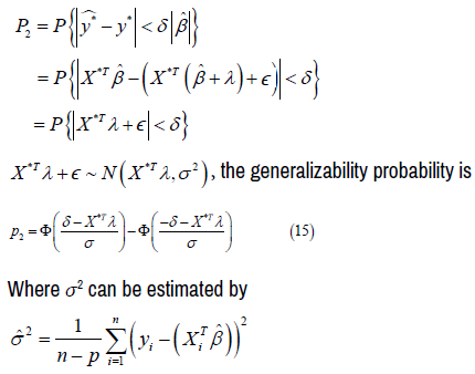
Adjusted approach 2 for generalizability: Similar to approach 1,
for approach 2, we replace  Then the expectation
  equates to
  The variance
  remains the same as it is in Eq. (3), given that the
added term
remains the same as it is in Eq. (3), given that the
added term  is a constant. Therefore, the distribution of
  becomes
  and the generalizability probability p2 is given by
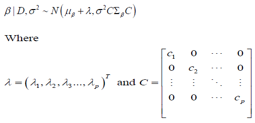
Adjusted approach 3 for generalizability: For approach 3, the Bayesian
method, the coefficients β are not fixed values but random variables assigned
to a probability distribution. Suppose the transition of regression coefficients
from the original population to a new population is characterized by a shift
of mean, denoted by λ and a recalibration of variance, denoted by  In other words,
  the distribution of the ith coefficient βi is replaced
by
the distribution of the ith coefficient βi is replaced
by  . Consequently, the covariance between βi and βj will
be scaled to
. Consequently, the covariance between βi and βj will
be scaled to  . Now we can construct a diagonal matrix C,
where the diagonal elements Cii = cii and non-diagonal elements are 0. The covariance matrix
. Now we can construct a diagonal matrix C,
where the diagonal elements Cii = cii and non-diagonal elements are 0. The covariance matrix  is then transformed into
  for a new, generalized
population.
for a new, generalized
population.
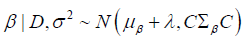
Therefore, under the premise that σ2 is known, the posterior distribution,
initially  undergoes a transition to
In the scenario that σ2 is unknown, the posterior distribution for β, initially  is modified to
Consequently, when σ2 is known, the posterior predictive distribution for a
similar but distinct population is given by substituting μβ+Σβ and respectively
for μβ and Σβ in Eq. (6), which results in  Thus,
the distribution for
Thus,
the distribution for  changes to
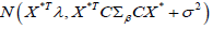
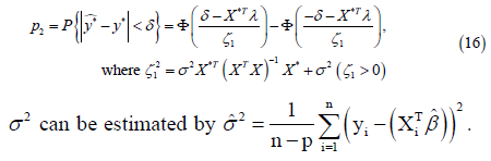
Then the generalizability probability p2 is estimated by

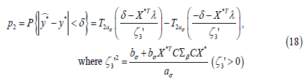
Similarly, for the cases when σ2 is unknown, replace μβ and Σβ with μβ+λ
and respectively and the posterior predictive distribution in Eq. (13)
becomes

The generalizability probability p2 is estimated by
In practice, when λ and C (or λ in approaches 1 and 2) are unknown, the
generalizability of the medical predictive model can be estimated by performing
a sensitivity analysis that calculates p2 based on a range of potential λ and C
(or λ) values. For example, if we want to assess the model's generalizability
when each regression coefficient may deviate by up to 10 percent from its
original value, we can take values of λi from the range  . These selected λi values are then used to construct a set of λ vectors. Using
these λ vectors, we compute a series of p2 values to evaluate the model's
capability in generalizing to data from new populations. The results of the
sensitivity analysis provide valuable insights into the model's applicability to
new patients, who come from populations distinct from the one upon which the
model was developed.
. These selected λi values are then used to construct a set of λ vectors. Using
these λ vectors, we compute a series of p2 values to evaluate the model's
capability in generalizing to data from new populations. The results of the
sensitivity analysis provide valuable insights into the model's applicability to
new patients, who come from populations distinct from the one upon which the
model was developed.
In this paper, we have summarized the procedure for developing a medical predictive model. Within the outline development process, we identify one critical issue that most of the medical predictive development in practice halts at the internal validation phase. Due to the lack of available data from new populations, there is a notable gap in external validation and assessment of the model's generalizability. To address this challenge, we propose methods for estimating the reproducibility and generalizability of medical predictive models. We first design three approaches to estimating the model’s reproducibility. Subsequently, methods for generalizability estimation are established by adjusting the three proposed methods. When the data of the new population is not accessible, our approaches allow for a sensitivity analysis that provides valuable insight into whether the model can be applied to patients from different populations. Under a validated medical predictive model, we are able to determine an optimal dose based on the risk factors included in the model for achieving the best clinical outcome for disease management. Such a model, one rigorously established and validated, can assist disease management from various aspects, including disease prevention, diagnosis, treatment, and clinical decision-making. Regarding future work, our approaches are proposed in the context of a linear regression model, where a closed-form solution for regression coefficients is utilized. Future opportunities to extend this research could aim to propose generalizability probability estimation methods for more complex modelling scenarios like logistic regression where a closed-form solution is not present.
None.
None.
Google Scholar, Crossref, Indexed at
Google Scholar, Crossref, Indexed at
Google Scholar, Crossref, Indexed at
Google Scholar, Crossref, Indexed at
Journal of Biometrics & Biostatistics received 3496 citations as per Google Scholar report