Evaluation of the Performance of High-Resolution Satellite Based Rainfall Products for Stream Flow Simulation

Dawit Girma^1* and Belete Berhanu^2
*Correspondence: Dawit Girma, College of Engineering and Technology, Wolkite University, Wolkite, Ethiopia, Tel: +251917736107, Email:

Keywords

•CHRIPS •SUFI-2 •SWAT •SWAT-CUP •TAMSAT

Introduction

A precise analysis of water resources issues (e.g., flood, drought, extreme events, socio-economic analysis) entails accurate measures/estimations of hydro climatic variables. For a comprehensive of the impact of rainfall on the environment, it is vital that one must use appropriate spatial and temporal resolution for rainfall measurements [1]. Satellite-based rainfall estimates with high spatial and temporal resolution and enormous areal coverage provided as a possible additional source of data for hydrological models in areas where conventional rain gauge measurements are not readily available, sparsely available and no radar for measuring representative rainfall magnitude [2,3]. These applications would even have far- reaching effects for several developing countries whose ground-based stations are sparse and no radar technology for measuring representative rainfall magnitude. However, there are errors associated with satellite-based rainfall which prompt several questions. How accurate are satellite-based rainfall products? Can high- resolution satellite rainfall products be used for hydrological applications? Focusing on this research questions needs coordinated efforts of scholars in different region of the world. Lack of knowledge on the accuracy of those satellite products is a challenge to the hydrological community especially under complex terrain. Therefore; it’s very important to assess the performance of these estimates. Several studies assessed the capability of satellite rainfall products for flow simulation capability using hydrological models. For instance, CMORPH, PERSIANN, and TRMM (TMPA) 3B42RT) and TMPA 3B42 data with rainfall station data for two medium-scaled watersheds of the Ethiopian highlands as input to the hydrological model. These results revealed 3B42RT and CMORPH simulations show reliable skills in their simulations but with small under estimation large flood peaks, while 3B42 and PERSIANN simulations have inconsistent capability. Also, this result showed the simulation based on the satellite-only product (3B42RT) gave a better performance than the satellite- gauge product (3B42RT). Regarding our country Ethiopia, some studies have been carried out to evaluate performance, validation, Inter-comparison of satellite-based rainfall products especially for Blue Nile basin e. g [4,5]. For instance, CMORPH, PERSIANN, and TRMM (TMPA) 3B42RT) and TMPA 3B42 data with rainfall station data for two medium-scaled watersheds of the Ethiopian highlands as input to the hydrological model. These results revealed 3B42RT and CMORPH simulations show reliable skills in their simulations but with small under estimation large flood peaks, while 3B42 and PERSIANN simulations have inconsistent capability. Also, this result showed the simulation based on the satellite-only product (3B42RT) gave a better performance than the satellite-gauge product (3B42RT [6]. Regarding our country Ethiopia, some studies have been carried out to evaluate performance, validation, Inter-comparison of satellite-based rainfall products especially for Blue Nile basin e. g [1,3,5] simulate stream flow [7]. Many satellite-based estimations of precipitation are out there in high spatial and temporal resolution, which makes them useful for distributed hydrological models [2]. However, not all the satellite rainfall estimates are suitable for all the areas (i.e., their suitability and performance vary from region to region [8]. There is, therefore, a requirement to quantify their uncertainties before selecting the acceptable product for the region [9]. Therefore, hydrologists are still uncertain in applying these products directly in hydrological applications knowing that a lot of uncertainties are still involved in such techniques [7,10]. This study intended to evaluate the performance of two widely used, high-resolution, easily available and highly suitable for fully and semi distributed hydrologic model; satellite rainfall datasets (namely, CHRIPS and TAMSAT) for simulating stream flow modeling in Genale.

Research Methodology

As a procedure we follow the following main approaches.1) Inter- comparison of satellite rain fall products with rain gauge data at daily, monthly and annual time scale using point- to -grid inter comparison method. In point- based inter-comparison methods, individual rainfall stations are compared with the grid-based satellite and reanalysis products, whereas, in the grid-to-grid inter-comparison, the observed rainfall are interpolated to the same resolutions of the selected grid-based satellite and reanalysis rainfall products and then evaluated. Grid to grid method of evaluation is appropriate where the area is covered with a high number and uniformly networked gauge stations. In areas with sparsely distributed and limited number of rain gauge stations and complex terrain as in the case of the present study, point to grid method is the best way to evaluate each satellite and reanalysis rainfall product independently using their native resolution. In the present study, both statistical indices and categorical statistical indices were adopted to evaluate the precision of the satellite rainfall products. 2) Simulation of steam flow with SWAT using satellite rainfall products. 3) Calibration and validation simulated stream flow with SWAT-CUP using observed steam flow. 4) Comparison of the performance of simulated steam flow obtained from calibration and validation.

Study area

Genale Dawa river basin lies in the southern part of Ethiopia, covering parts of Oromia, SNNP, and Somali regions. Geographically located between 30 30' and 70 20' North latitude and 37005' and 430 20' East longitude. The basin covers an area of 172889 km². It is the third-largest river basin, after Wabi Shebelle and Abbay river basins. Neighboring river basins are the Wabi Shebelle to the north and east, Rift Valley basin to the west. Genale Dawa river basin have very scarce metrological station and Mountainous topography and provided as area where satellite rainfall products are beneficiary. The climate of the country is mainly controlled by the seasonal migration of the Inter- tropical Convergence Zone (ITCZ), which is conditioned by the convergence of trade winds of the northern and southern hemisphere and the associated atmospheric circulation. It is also highly influenced, regionally and locally, by complex topography of the country.

High resolution satellite rainfall products

In this study two high-resolution, satellite-based rainfall estimations that are available at high resolution (1 d, 0.037 × 0.037): TAMSAT and (1 d, 0.05 × 0.05): CHRIPS. We use the satellite data set as input at daily time scale.

SWAT model

SWAT needs Soil, Land use and DEM to drive flows and sub-watershed.These data are spatially distributed but SWAT lumps the parameter into hydrologic response units. Hydrologic response units (HRUs) that have unique land use, soil, and slope. The land use, soil, and slope datasets were projected into the same projections as DEM. After projection of the land use, soil, and slope datasets were reclassified, overlapped and connected with the SWAT catalogs and ready for HRU definition. The minimum threshold area of 10% for land use, 10% for soil class and 10% for slope were used. The land use, soil and slopes percentage areas covering less than the threshold area level were eliminated, and then the remaining areas were reclassified so that a hundred percent of the land area in the sub-basin could be used in the simulation execution.

Parameter specifications

The sensitivity analysis was made using a built-in SWAT sensitivity analysis tool that uses the Latin Hypercube One-factor-At-a-Time (LH-OAT) [11]. The inputs were the observed daily flow data, the simulated annual flow data and the sensitive parameter in relation to flow with the absolute lower and upper bound and default type of change to be applied (method application) were used. Latin Hypercube One-factor-At-a-Time (LH-OAT) combines the OAT design and LH sampling by taking the Latin Hypercube samples as initial points for OAT design. The Latin Hypercube One-factor-At-a-Time (LH- OAT) sensitivity analysis method combines thus the robustness of the Latin Hypercube sampling that ensures that the full range of all parameters has been sampled with the precision of an OAT designs assuring that the changes in the output in each model run are often unambiguously attributed to the input changed in such a simulation resulting in a strong and efficient sensitivity analysis method [11] (Table 1).

Calibration

After the selection of most sensitive parameter, we carried out auto calibration through Sequential Uncertainty Fitting algorithm (SUFI-2) imbedded in SWAT-CUPIn SUFI-2, parameter uncertainty accounts for all sources of uncertainties such as uncertainty in driving variables (e.g., rainfall), conceptual model, parameters, and measured data [12]. The intelligence of SWAT-CUP allows model parameters to be predefined and optimized throughout the auto-calibration process or manually adjusted iteratively between calibration batches [13]. Among various evaluation coefficients contained in SUFI-2, Nash-Sutcliff (NSE) was selected for model optimization in SWAT-CUP.

Model performance evaluation

To evaluate the model simulation outputs relative to the observed data, model performance evaluation is necessary. There are various methods to evaluate the model performance during the calibration and validation periods. For this study, the objective functions to measure the model's goodness of fit for discharge was Nash-Sutcliffe Efficiency (NSE), Determination coefficient (R2), The Root Mean Square Error (RMSE), and PBIAS. In the present study, both statistical indices and categorical statistical indices were adopted to evaluate the precision of the satellite rainfall products. Statistical indices evaluate the performance of the Satellite rainfall product in estimating the cumulative rainfall over a timeframe. The statistical indices are:

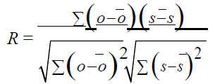
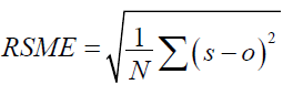
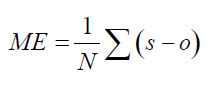
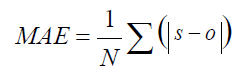
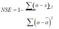
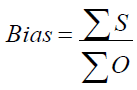
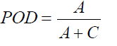
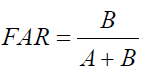
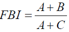
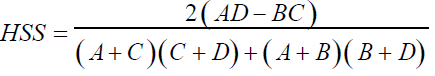
Where O is that the total observed rainfall, O ̅ is that the mean observed rainfall, S is a satellite rainfall product, and N is the number of data pairs compared. The measure of ME and MAE are in mm, whereas NSE and Bias are unit less. ME and MAE both provides information on the typical estimation error. ME ranges from –∞ to ∞, whereas MAE ranges from 0 to ∞, and an ideal score for both is 0. MAE was used here instead of the root mean square error to avoid the effect of extremely high rainfall values or outliers [14]. The Bias statistic indicates how well the mean estimate and gauge mean correspond; its value ranges from 0 to ∞, with 1 being an ideal score. Values of Bias >1 and positive ME values indicate an overestimation, whereas values of Bias <1 and negative ME indicate an underestimate. NSE shows the skill of the estimates relative to a reference (in this case, the mean of the gauge observations); it ranges from –∞ to 1, with higher values indicating better agreement between the Satellite rainfall and gauge measurements. Negative NSE values indicate that the reference mean may be a better estimate than the SREs; 0 indicates that the reference mean is nearly as good as the Satellite rainfall. A categorical statistical index evaluates the rainfall detection capabilities of satellite rainfall product. For the evaluation of the rainfall detection capabilities of the Satellite rainfall product (rainfall threshold ≥1 mm), we used a suite of binary skill scores that encapsulated information on rain/no-rain days in a contingency table (Table 2). The contingency table was constructed to compute categorical statistics that included the probability of detection (POD), false alarm ratio (FAR), frequency bias index (FBI), and Heidke skill score (HSS) as follows:

Where A, B, C, and D represent hits (the satellite successfully detected rain), false alarms (the satellite did detect the no-rain case), misses (the satellite did not detect rain), and correct negatives (the satellite successfully detected the no-rain case), respectively (Table 3). POD quantifies the proportion of observed rainfall days that were correctly estimated by the satellite product. FAR is that the proportion of satellite-estimated rainfall days when there was in fact no rain. Both POD and FAR range from 0 to 1, with 1 being an ideal POD and 0 being an ideal FAR. FBI, which ranges from 0 to ∞, compares the rainfall-day detection frequency of the Satellite rainfall product with that of the rain gauge measurements: an FBI of less than (greater than) 1 indicates an underestimate (overestimate) of rainfall days. HSS, which ranges from –∞ to 1, is a measure of the overall skill of the rainfall-day estimates after rain events detected by random chance have been removed: an HSS less than 0 indicates that random chance is better than the Satellite rainfall product; an HSS of 0 means the Satellite rainfall product has no skill; and an HSS of 1 indicates an ideal estimation of rainfall days by the Satellite rainfall product.

Results and Discussion

a) Comparison of rainfall input

Excellent performance of a product for rainfall detection would be characterized by a combination of high POD, high FBI, low FAR, and high HSS. For all the selected stations, TAMSAT had the lower rainfall detection skill: compared to CHRIPS. It truly identified more than 71.62% of the observed rainy days (POD). While, CHIRPS had the highest rainfall detection skill: it correctly dictates more than 81% of the rainfall events for all the selected stations. The POD values reveal that both the SREs missed moderate rainfall events in all the nine selected stations. FAR values indicated that around 22% and 5% of the estimated rainy days were falsely estimated by the TAMSAT and CHRIPS respectively. In general, FAR was relatively low for all the selected stations. FBI values were 86% and 92.1% for CHIRPS and TAMSAT respectively, an indication that these two SREs underestimated the frequency of rainfall. The main problem with the SREs over the study region therefore seems to be the moderate overestimation (TAMSAT) and underestimation (CHIRPS) of rainfall occurrence. The HSS values were high, the implication being that the skill of the SREs in detecting rainfall occurrences was much better than random chance. Generally, CHRIPS demonstrates better rainfall detection capability on most of the evaluation metrics compared to TAMSAT over all the selected stations (Table 3).

At a daily time scale the ME was small relative to the average daily rainfall (O ¯) for both the SREs. There were small random errors in the TAMSAT estimates for all the selected stations, as indicated by the lower ME values 0.05 and -0.44 for TAMSAT and CHRIPS respectively. TAMSAT and CHIRPS estimated the amount of rainfall reasonably well (high efficiency, low random errors, and bias <10%) at daily time scales. The better accuracy of the TAMSAT estimates may have resulted from the use of thresholds that varied spatially and temporally and from the high temporal resolution. The fact that TAMSAT is bias-adjusted, and CHIRPS is bias-adjusted and includes contemporaneous station data could also result in better rainfall estimation. CHIRPS had the NSE and R (> 0.75, >0.88) respectively and TAMSAT had the NSE and R (> 0.76, >0.88) respectively. All the evaluation statistics confirm that TAMSAT and CHIRPS performed better and the differences in the evaluation statistics between TAMSAT and CHIRPS were very small for all selected stations.

Inter-comparison of daily rainfall estimates. The comparison statistics (R = Pearson’s correlation coefficient) are given in each plot. Correlations between satellite rainfall values and rain gauge values were very good which ranges (0.8064 – 0.9614) for CHRIPS and (0.827-0.951) for TAMSAT (Figures 1-3).

Inter-comparison of mean monthly rainfall data for rainfall estimates. The mean monthly maximum rainfall has the same trend as observed data. The rainfall maximum is in April with a secondary maximum in October for each location and the minimum are in January and July for each location. Compared to rain gauges values, CHRIPS satellite rainfall products underestimated the monthly rainfall in the range 0.84% to 28.5%, While TAMSAT over estimated in the range 0.52% to 30% (Figure 4). Inter-annual variation of rain observed by rain gauges was generally captured by both of satellite rainfall products for all selected stations. The CHRIPS product shows a small underestimation of annual maximum rainfall for the whole study period and all selected station from 39.9 to 6938.8 mm/yr. But shows better performance in capturing inter- annual variation of rainfall. TAMSAT product shows overestimation of annual maximum rainfall from 84.4 to 2054.81mm/yr. for the whole study period when compared with Observed data (Figure 5). In capturing both magnitude and trend of annual rainfall bias corrected TAMSAT shows better performance.

The above comparison, especially the daily basis is very important in our case because Arc SWAT uses daily observed rainfall data. Therefore, both CHRIPS and TAMSAT rainfall estimates gave a very good result, and this result also consistent with findings in Eastern parts of Ethiopia [15,16]. There have been subsequent studies that conducted in Ethiopia to evaluate satellite rainfall products in the estimation of rainfall [17-19]; based on their studies and the result of this study, it is concluded that TAMSAT and CHRIPS are much closer to the actual rainfall fields in Ethiopian basins [1,3].

b) Model simulation, calibration and validation

Base flow and surface flow were separated using the automated digital filter methods based on the daily flow data measured at the outlet. The base flow separation technique indicated that about 29.8% of the total water yield was contributed from the subsurface water source which was less than surface runoff involvement for the total water yield at the outlet of the watershed for CHRIPS product and 29% of the total water yield was contributed from the subsurface water source which was again less than surface runoff involvement for the total water yield at the outlet of the watershed for TAMSAT. The average value of CN of the sub-basin lies between 75.57 and 86.22 for CHRIPS and 83.36 and 87.16 for TAMSAT model. The value of saturated soil conductivity can also affect groundwater flow. Consequently, this maximum value of CN2 and moderate conductivity SOL_K indicates flow to be surface flow dominated. Percent of error of the observed and simulated daily flows at the selected gauge stations are (2.8 - 8.2)% for CHRIPS product and (-11.6 - 3.6)% for TAMSAT product which is well within the acceptable range of ±15%. Further a good agreement between observed and simulated daily flows are shown by the coefficient of determinations (R2 =0.84 - 0.88) for CHRIPS and (R2 =0.71 - 0.95) for TAMSAT and the Nash-Suttcliffe simulation efficiency (NSE=0.78-0.86) for CHRIPS and (NSE=0.7 - 0.92) for TAMSAT thus fulfilled the requirements for R >0.6 and ENS> 0.5 (Figure 6).

Validation of the model was carried out and the percent of error between the observed and simulated daily flow are (-0.82 - 3)% for CHRIPS and (-14 - 0.3)% for TAMSAT. Thus, it is found within the tolerable range of ±15%. The coefficient of determinations (R2) was found to be (0.72 - 0.93) for CHRIPS and (0.81 -0.87) for TAMSAT respectively and Nash-Sutcliffe simulation efficiency (NSE) was (0.7 - 0.95) for CHRIPS and (0.76 -0.88) for TAMSAT respectively (Figure 7). These shows a very good correlation of the simulation results with the observed values.

Generally, there is a good fit between measured and simulated output and a slight over estimation of the low flows and under estimation of the peak flows were observed at the validation period. Since the model performed as well in the validation period, as for the calibration period hence, the set of optimized parameters listed in Table 3 and Table 4 during calibration process for Genale Dawa River Basin can be taken as the representative set of parameters for the basin. Thus, the validation check illustrates the accuracy of the model for simulating time-periods outside of the calibration period. The model performed as good in the validation period (2004-2007), as for the calibration period (1998-2003) at the four-gauge stations as indicated in Table 4. Hence, the set of optimized parameters used during calibration process can be taken as the representative set of parameters to explain the hydrologic characteristic of the Genale Dawa River Basin and further simulations using SWAT model can be carried out by using these parameters for any period of time.

Similar study conducted by Samuel [20] reported that the results of testing and verification of the model at monthly time pace gave NSE of 0.65, Pbias of 15 and RSR of 0.4, while E of 0.5, Pbias of 31 and RSR of 0.5 were recorded for validation. Shawul A. Alemayehu et al. [21] reported R² of 0.86 and NSE of 0.85 for calibrated monthly flows, and for validation the following monthly flows statistics were reported as R² of 0.69 and NSE of 0.61. Ruan, Hongwei et al. [22] reported R2 of 0.75 and NSE of 0.74 for calibrated monthly flows, and for validation the following monthly flows statistics were reported as R² of 0.58 and NSE of 0.69. Shawul A. Alemayehu et al. [23] reported R² of between 0.62 and 0.84 and NSE of between 0.41 and 0.84 for calibrated monthly flows. Bayissa, Yared et al. [17] noted R² of 0.80 and NSE of 0.73 for calibrated while R² of 0.80 and NSE of 0.71 for validation period. In an interrelated study also reported by Shawul A. Alemayehu [21] that the SWAT model had a worthy demonstration in replicating the stream flow with the R², NSE and percent difference values of 0.81, 0.75 and 23 respectively in the testing period, while R², NSE and percent difference values of 0.65, 0.59 and 20 respectively in the verification [24] period. There is some variation in statistical values among researchers, in this particular study too, this variation might be due to mainly spatial data used (predominantly land use land cover data), disparity in catchment sensitive parameters that affect calibration processes, uncertainty during data handling and due many more cases.

Discussion and Conclusion

The study "Evaluation of the performance of high-resolution Satellite rainfall product for stream flow simulation was conducted as a case study of Genale Dawa River basin. The basin can be provided as a good example where the use of satellite-derived precipitation could be beneficial. To overcome limitation of lacking sufficient station data, this research study uses some of the available globally gridded high resolution precipitation datasets to simulate runoff using SWAT model. Two satellite precipitation products (CHRIPS and TAMSAT) were selected for this evaluation.

The products were evaluated and compared on daily, monthly and annual time scales against the ground precipitation measurements through visual assessment of plots and by using some statistical methods such as Nash- Sutcliffe Coefficient of Efficiency, root mean square difference, estimation bias, and correlation coefficients and so on. The comparison results of rainfall magnitudes from satellite rainfall products and rain gauges revealed that the CHRIPS and bias corrected TAMSAT rainfall estimates gave relatively accurate result compared to rain gauge rainfall estimates at daily scale. Comparing CHRIPS and bias corrected TAMSAT, the former shows better result. The result revealed that, in this region, correlations between satellite rainfall values and rain gauge values were good (R Values are ranging from 0.72 to 0.96) for different selected stations.

On comparison of monthly datasets, the trend is totally captured while the magnitude shows under estimation from 5.7% to 30% by CHRIPS product and shows small over estimation from 0.75% to 3.4% for TAMSAT product. On the basis of annual comparison our result showed that tend correctly captured and CHRIPS shows small under estimation while TAMSAT shows small over estimation. Our results reveal that the utility of satellite rainfall products as input to SWAT for daily stream flow simulation strongly depends on the product type.

Simulation from both rainfall inputs showed the trend of observed hydrograph. Simulation based on CHRIPS and TAMSAT showed consistent and modest skills in their simulations. Overall, the results indicate that although some uncertainties exist in these gridded datasets (CHRIPS & TAMSAT), the appliance of these gridded data prove useful for hydrological studies within the absence of station data. When comparing simulation from both inputs, R2 ranges from 0.72 to 0.97 for CHRIPS and from 0.71 to 0.95 for TAMSAT during calibration and validation. The NS ranges from 0.7 to 0.95 for CHRIPS and from 0.7 to 0.92 for TAMSAT. It strongly indicates the raising potential of the predictive accuracy of the satellite rainfall products in reproducing hydrological features. The SWAT model also proves to be a good tool in such a modeling approach. In all cases the bias corrected TAMSAT shows better results compared to CHRIPS.

Data Access and Format

The daily rainfall estimates (in mm per day) are freely available as net CDF files for each day from the TAMSAT website (http://www.tamsat.org.uk) and the University of Reading Research Data Archive. The spatial resolution is 0.0375° latitude by 0.0375° longitude with estimates provided for all land points in Africa, including Madagascar. In addition, the TAMSAT website contains quick look images for each day and a time series extraction tool can be used to extract area-average data for countries, administrative districts and user defined rectangular regions or user defined pixels in csv format. Climate Hazards Group Infrared Precipitation with Stations (CHIRPS) with a relatively high spatial and temporal resolution (i.e., 5 km resolution at daily temporal scale) and quasi-global coverage from January 1981 onwards. This product is accessed from (http://ftp.chg.ucsb.edu). The weather input data required for SWAT simulation includes daily data of Precipitation, maximum and minimum temperature, relative humidity, wind speed, and solar radiation. These were obtained from the Ethiopian National Meteorological Agency. The weather data used were represented from six stations inside Genale Dawa River basin. The climatic data used for this study covers 22 years from January 1996 to December 2017. Stream flow data used for calibration and validation of the model were collected from Ethiopian ministry of water and electricity. It covers 10 years (1998-2007); six years for calibration and four years for validation.

References

1. Ayehu T. Getachew, Tsegaye Tadesse, Berhan Gessesse and Tufa Dinku. "Validation of new satellite rainfall products over the Upper Blue Nile Basin, Ethiopia." Atmos. Meas. Tech 11 (2018): 1921-1936.
2. Chad Furl, Dawit Ghebreyesus and Hatim O Sharif. “Assessment of the Performance of Satellite-Based Rainfall product overupper Blue Nile river basin.” Geosci (2018): 1-18.
3. Dinku T, P. Ceccato, E. Grover‐Kopec, M. Lemma and S. J. Connor, et al. "Validation of satellite rainfall products over East Africa's complex topography." Int. J. Remote Sens 28 (2007): 1503-1526.
4. Gebere B. Shimelis, Tena Alamirew, Broder J. Merkel and Assefa M. Melesse. "Performance of high resolution satellite rainfall products over data scarce parts of Eastern Ethiopia." Remote Sens 7 (2015): 11639-11663
5. Bitew M. Menberu, Mekonnen Gebremichael, Lula T. Ghebremichael and Yared A. Bayissa. "Evaluation of high-resolution satellite rainfall products through streamflow simulation in a hydrological modeling of a small mountainous watershed in Ethiopia." J. Hydrometeorol 13 (2012): 338-350
6. Funk C. Chris, Pete J. Peterson, Martin F. Landsfeld and Diego H. Pedreros, et al. "A quasi-global precipitation time series for drought monitoring." U.S. Geol. Surv. 832 (2014): 1-12.
7. Fenta A. Ayele, Hiroshi Yasuda, Katsuyuki Shimizu and Yasuomi Ibaraki, et al. "Evaluation of satellite rainfall estimates over the Lake Tana basin at the source region of the Blue Nile River." Atmos. Res 212 (2018): 43-53
8. Sahlu Dejene, Semu A. Moges, Efthymios I. Nikolopoulos and Emmanouil N. Anagnostou, et al. "Evaluation of high-resolution multisatellite and reanalysis rainfall products over East Africa." Adv. Meteorol 2017 (2017)
9. Gella W. Getachew. "Statistical evaluation of High Resolution satellite precipitation products in arid and semi‐arid parts of Ethiopia: a note for hydro‐meteorological applications." Water Environ J 33 (2019): 86-97.
10. Bitew M. M and Gebremichael M. “Assessment of satellite rainfall products for streamflow simulation in medium watersheds of the Ethiopian highlands. Hydrol. Earth Syst. Sci. 15(2011): 1147-1155.
11. Neitsch L. Susan, Jeffrey G. Arnold, Jim R. Kiniry and Jimmy R. Williams. Soil and water assessment tool theoretical documentation version 2009. Texas Water Resources Institute, 2011.
12. Abbaspour C. Karim, M. Vejdani, S. Haghighat and J. Yang. "SWAT-CUP calibration and uncertainty programs for SWAT." In MODSIM 2007 international congress on modelling and simulation, modelling and simulation society of Australia and New Zealand (2007); 1596-1602.
13. Ha T. Lan, Wim GM Bastiaanssen, Ann van Griensven and AlberT IJM Van Dijket, et al. "SWAT-CUP for calibration of spatially distributed hydrological processes and ecosystem services in a Vietnamese river basin using remote sensing." Hydrol. Earth Syst. Sci (2017): 1-35.
14. Legates R. David and Gregory J. McCabe Jr. "Evaluating the use of “goodness‐of‐ fit” measures in hydrologic and hydroclimatic model validation." Water Resour. Res 35 (1999): 233-241.
15. Tolera, Mesfin Benti, Il-Moon Chung and Sun Woo Chang. "Evaluation of the climate forecast system reanalysis weather data for watershed modeling in Upper Awash basin, Ethiopia." Water 10 (2018): 725.
16. Basheer, Mohammed, and Nadir Ahmed Elagib. "Performance of satellite-based and GPCC 7.0 rainfall products in an extremely data-scarce country in the Nile Basin." Atmos. Res 215 (2019): 128-140.
17. Bayissa, Yared, Tsegaye Tadesse, Getachew Demisse and Andualem Shiferaw. "Evaluation of satellite-based rainfall estimates and application to monitor meteorological drought for the Upper Blue Nile Basin, Ethiopia." Remote Sens. 9 (2017): 669.
18. Young P. Matthew, Charles JR Williams, J. Christine Chiu, Ross I. Maidment and Shu-Hua Chen. "Investigation of discrepancies in satellite rainfall estimates over Ethiopia." J. Hydrometeorol 15 (2014): 2347-2369.
19. Dinku Tufa, Kinfe Hailemariam, Ross Maidment and Elena Tarnavsky, et al. "Combined use of satellite estimates and rain gauge observations to generate high‐ quality historical rainfall time series over Ethiopia." Int J Climatol 34 (2014): 2489 - 2504.
20. Tetsoane T Samuel. “Evaluation of the SWAT Model in Simulating Catchment Hydrology: Case Study of the Modder River Basin”: M.Sc. thesis, Central University of Technology, Free State, South Africa., 2013.
21. Shawul A. Alemayehu, Tena Alamirew and M. O. Dinka. "Calibration and validation of SWAT model and estimation of water balance components of Shaya mountainous watershed, Southeastern Ethiopia." Hydrol. Earth Syst. Sci. Discuss 10 (2013): 13955-13978.
22. Ruan, Hongwei, Songbing Zou, Zhentao Cong and Yuhan Wang, et al. "Runoff simulation by SWAT model using high-resolution gridded precipitation in the upper Heihe River Basin, Northeastern Tibetan Plateau." Hydrol. Earth Syst. Sci. Discuss (2016):866.
23. Shawul A. Alemayehu, Tena Alamirew, Assefa M. Melesse, and Sumedha Chakma. "Climate change impact on the hydrology of Weyb River watershed, Bale mountainous area, Ethiopia." In Landscape dynamics, soils and hydrological processes in varied climates. Springer, Cham, 2016: 587-613.
24. Setegn and Shimelis Gebriye. "Modelling hydrological and hydrodynamic processes in Lake Tana Basin, Ethiopia." PhD diss., KTH, 2010.