Research Article - (2021) Volume 0, Issue 0
Received: 15-Sep-2021
Published:
07-Oct-2021
, DOI: 10.37421/bset.2021.S1.003
Citation: Shinobu Ishigami, Ken Kawamata. "Measurement Technique and Antenna / Sensor for Transient Electromagnetic Fields Caused by Electrostatic Discharge." J Biomed Syst Emerg Technol S1 (2021): 003.
Copyright: © 2021 Ishigami S, et al. This is an open-access article distributed under the terms of the Creative Commons Attribution License, which permits unrestricted use, distribution, and reproduction in any medium, provided the original author and source are credited.
A transient electromagnetic field caused by an electrostatic discharge (ESD) is a serious noise source for electric equipment / system especially such as digital equipment. Therefore, it is an important issue in electromagnetic compatibility (EMC). In this paper, we introduced the measurement technology of the wideband transient electromagnetic field generated by the ESD phenomenon. By converting the waveform observed by the oscilloscope into the frequency domain using the discrete Fourier transform, removing the characteristics of the measuring apparatus such as the broadband amplifier measured by the S-parameters, and applying the complex antenna factor of the antenna / sensor. These data were converted using the inverse Fourier transform, then the real waveforms of the electromagnetic field were obtained. We also introduced antenna / sensor calibration methods specialized for the far field and the near field, and examples of their characteristics. In particular, the usefulness of a broadband folded long-hexagon antenna for far-field measurement was shown.
Electrostatic discharge (ESD) • Measurement method• Broadbrand Antenna
An electrostatic discharge (ESD) is generated by collision or contact between charged objects, and an impulsive transient electromagnetic field with a wide frequency range is radiated. For information and telecommunications equipment, which has been digitized in recent years, an impulsive electromagnetic noise may induce erroneous processing of information signals and may interfere with the normal operation of the system. On the other hand, inside the systems of information and communications, electronic circuits are becoming more integrated and minimalize, the voltage of operating signals is decreasing, and the operating speed is increasing. Therefore, these systems tend to be particularly susceptible to the impulse electromagnetic noise such as ESD fields, and it is an important issue in electromagnetic compatibility (EMC) [1-6]. This paper describes how to measure the above-mentioned the ESD transient electromagnetic fields in the time domain. In addition, the characteristics and shape of a newly developed ultra-wideband antenna as an antenna for use in ESD transient electromagnetic field measurements are introduced.
A. Definition of complex antenna factor
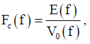
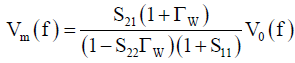
In the area of EMC measurements, the antenna factor is usually used as a conversion factor between the detected electric field and the antenna terminal voltage. To maintain a compatibility with the conventional antenna factor, phase information is added to this factor to define a "complex antenna factor" [7]. When the antenna is installed in a plane wave as shown in (Figure 1) the complex antenna factor Fc(f) is defined by the following equation.

Figure 1. Definition of complex antenna factor.
 (1)
(1)
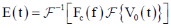
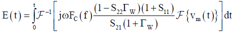
Where E(f) is the complex electric field on elements of the antenna with a certain frequency f, and V0(f) is the matched output voltage of the antenna for the characteristic impedance Z0. Since V0(f) is obtained by the Fourier transform for the waveform of the matched output voltage V0(t) and the electric field waveform E(t) is obtained by the inverse Fourier transform for E(f), the field waveform E(t) can be expressed by next.
 (2)
(2)
Where  and
and  denote the Fourier and the inverse Fourier transforms, respectively.
B. Measurement Method of Complex Antenna Factor
There are three main methods for measuring the (complex) antenna factor of an antenna as follows.
(a) Standard field method
(b) Reference antenna method
(c) 3-antenna method
The standard field method is a technique in which an antenna to be calibrated is installed at a point where the electric field strength at a certain distance is known and the antenna factor is obtained. That is, the amplitude of the electric field E(f) is known, and the amplitude of the antenna factor  is obtained by measuring the amplitude of the matched output voltage of the antenna to be calibrated in (1). A known electric field is generated by using an antenna whose gain is known in advance by a calculation or calibration. The standard field method can also be applied with an electric field generated by a TEM cell.
In the reference antenna method, an antenna whose antenna factor  is known is prepared. The antenna is called as a reference antenna. At the first, the reference antenna is installed in a place where a steady electromagnetic field is generated, and the matched output voltage of the antenna
  is measured. Next, the reference antenna is removed, an antenna to be calibrated is installed in the same place, and the matched output voltage of the antenna is measured. The amplitude of the antenna factor of the antenna to be calibrated
  is calculated using the following equation.
 (3)
(3)
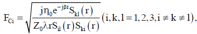
(Equation 3) shows the antenna factor to be obtained does not depend on the electric field strength. Therefore, even if the exact electric field strength of the transmitting antenna that generates the electromagnetic field is unknown, the antenna factor of the antenna to be calibrated can be obtained by this method. However, it is difficult to obtain the phase information of the complex antenna factor by the methods (a) and (b). In addition, the methods (a) and (b) require an antenna with known antenna gain or antenna factor. With the 3-antenna method, the antenna factor can be obtained without preparing an antenna with the known gain or antenna factor, and when a vector network analyzer (VNA) is used for the measurement, the complex antenna factor with the phase information can be obtained. The principle of the 3-antenna method is shown in (Figure 2). This method is an antenna calibration method that does not require a primary standard antenna with a known antenna factor or an antenna gain. However, the measurement in the method usually performed in an anechoic chamber because the method is easily affected by the measurement environment. In this method, three antennas are alternately used as transmitting / receiving antennas, and three types of propagation S-parameters Ski (i, k =1, 2, 3, where i ≠ k) are measured by a VNA. Using these three propagation S-parameters, the complex antenna factor Fci of each antenna can be calculated by the following equation.

Figure 2. Schematic of the 3-antenna method.
 (4)
(4)
Where 0 j, η , β, r, λ are the imaginary unit, the wave impedance in free space (=120π [Ω]) the propagation constant between the transmitting and receiving antennas, the distance between the transmitting and receiving antennas in meters, and the wavelength in meters, respectively.
C. Measurement of Complex Antenna Factor
This subsection shows an example of the measurement result of the complex antenna factor measured by the 3antenna method. (Figure 3) shows a monopole antenna for the measurement as an example. (Figure 4) shows the frequency response of the measured complex antenna factors for the monopole antenna. (Figure 5) shows the values obtained by multiplying the complex antenna factor at each frequency by jω (corresponding to the time derivative in the time domain). The reason for obtaining this value will be explained in the next subsection.

Figure 3. Structure of a monopole antenna.

Figure 4. Example of complex antenna factor (amplitude).

Figure 5. Product of complex antenna factor and jω (amplitude and phase).
D. Waveform Reconstruction Technique
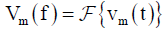
This subsection describes a reconstruction method of electric-field waveform using the complex antenna factor taking the case of observing the electric field waveform by an ESD event with the monopole antenna in the previous subsection as an example. The path from an antenna output to an oscilloscope input has a suite of devices such as a broadband amplifier, attenuators, and cables intervening in the path as shown in (Figure 6). Therefore, the waveform observed by the oscilloscope includes the propagation and reflection characteristics of the devices and the antenna. To obtain an accurate electric-field waveform, the characteristics of these devices and antenna shall be removed from the observation data obtained by the oscilloscope. If the waveform recorded by the oscilloscope is Vm(t), the voltage Vm(f) at a certain frequency f is expressed by the following equation using the Fourier transform.

Figure 6. Example of waveform measuring apparatus.
 (5)
(5)
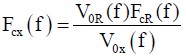
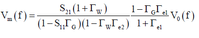
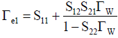
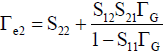
When the characteristics of such devices are collectively expressed by S-parameters, and these parameters and reflection coefficients are defined as described in (Figure 6), Vm(f) in the frequency domain is expressed by the following equations.
 (6)
(6)
 (7)
(7)
 (8)
(8)
In the example of (Figure 6), the reverse propagation S-parameter S12 is negligibly small due to the presence of the amplifier. In that that case, Vm(f) becomes simpler as follows.
 (9)
(9)
On the other hand, when using a linear antenna such as a dipole antenna or a monopole antenna for electric field measurement, the complex antenna factor increases as the frequency decreases and diverges infinitely at f = 0 (DC). (See Figure 4). In this case, the time derivative waveform of the electric field is obtained from Eq.(2) using the value obtained by multiplying the complex antenna coefficient by jω (corresponding to the time derivative in the time domain) (see Figure 5). The electric-field waveform itself can be reconstructed by first-order integrating the waveform with respect to time. The reconstructed waveform is expressed as the following equation by applying (Equation 9) to (Equation 2).
 (10)
(10)
In the waveform reconstruction by (Equation 10), the goal is not to obtain the spectrum of the electromagnetic field, but to reconstruct the electric or magnetic field waveform. Therefore, if the original observed waveform is excessively deformed by a time window function normally used when obtaining the spectrum, the reconstructed waveform may be distorted. There are several ways to avoid such distortion listed below.
(1) Increase the observation time and measure so that the target part comes to the center of the waveform. For example, as shown in the upper figure of (Figure 7), the main part of the waveform should be measured so that it fits in about 60 % of the center of the waveform data. In addition, a processing is performed so that the time window function is smoothly applied to 20% before and after the waveform data.

Figure 7. Processing of observed waveforms for waveform.
(2) In the case of a stepped waveform as shown in the lower figure of (Figure 7), the values of the start time and end time of the acquired waveform are different. If the gradients of the waveforms are mostly equal to each other at the start and end times, first differentiated in the time domain (actually, taking the difference because the data are discrete) should be conducted for the original waveform. After the processing in the frequency domain and the inverse Fourier transform, an integral calculation is performed again in the time domain.
It is also necessary to pay attention to the frequency components of the acquired data. Since the data is usually acquired using a digital oscilloscope, the sampling and quantization for the data will be already completed. Assuming that the number of samples is n and the total time of the acquired waveform is T, the time interval (sampling period) Δt in sampling is given by the following equation.
 (11)
(11)
According to the Nyquist theorem, the highest frequency fmax of the sampled data is expressed as (Equation 12), and the sampling frequency fs is as in (Equation 13).
 (12)
(12)
 (13)
(13)
According to Shannon-Someya's sampling theorem, the sampling frequency shall be at least twice the highest frequency contained in the data. If the original data contains frequencies above fs/2, it is necessary to pass it through a low-pass filter (LPF) before sampling. If the bandwidth of a waveform observation device such as an oscilloscope is lower than that of fs/2 and the frequency level above fs/2 is sufficiently low, the LPF is not always necessary. A frequency interval Δf in the frequency domain after the Fourier transform is obtained as follows.
 (14)
(14)
Frequency intervals of the S-par ameters of the measuring devices and the complex antenna factors of the antenna should be chosen to the interval Δf shown in Eq (14) for later processing. Considering the operations in the Fast Fourier Transform (FFT), it is convenient to select the number of the sample n to the power of 2. If the maximum frequency fmax of the data is lower than the highest frequency of the S-parameters of the measuring instruments or the complex antenna factor of the antenna (Sji or Fc(f) in (Equation 10), the data of the S-parameter and complex antenna factor should be used up to fmax. On the contrary, when the highest frequency of the measuring instruments is lower than fmax, and there is no data more than fmax the S-parameters and complex antenna factor at the unmeasured frequency should be set to 0. Such process can avoid division by zero occurring in the calculation. A method should be used in which the waveform spectrum data above the highest frequency of the measuring instruments is forcibly set to 0, or the level near the highest frequency of the measurement is gradually attenuated.
As an example, a waveform observed by a discharge experimental apparatus stated in [8] including an oscilloscope and the monopole antenna (See Figure 3) is shown in (Figure 8). The reconstructed electric-field waveform from the observed waveform is shown in (Figure 9). In the figure, an electrostatic field of about -1.7 kV/m is generated between the discharge electrode and the ground plane until just before the time of 3 ns. In addition, the electric field strength suddenly changes in a pulse shape toward 0 V/m due to the discharge caused by the breakdown of the air insulation.

Figure 8. Observed waveform obtained by an oscilloscope.

Figure 9. Example of reconstructed electric-field waveform.
This section introduces a minimally invasive optical electric-field sensor (OES) used to measure transient electricfield waveforms in the vicinity of the discharge electrode and explains a calibration technique of the antenna factor of the sensor. The sensor introduced in this section is a minimally invasive OES (SEIKOH GIKEN: C3-1055 with CS-1210, 100 kHz-10 GHz). The antenna factor of the sensor is around 65 dB/m at frequencies of 1 MHz or higher according to the manufacturer's specifications. To confirm the factor given by the manufacturer, the antenna factor of the sensor was calibrated using a TEM cell (Elena ETC-805W) as shown in (Figures 10 and 11) shows a setup for calibration of the sensor using the TEM cell.

Figure 10. TEM cell for calibration of optical E-field sensor (OES).

Figure 11. Setup for calibration of OES using TEM cell.
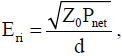
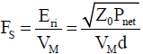
The OES under calibration is positioned so that a septum (center conductor) of the TEM cell and the midpoint of the distance between the ceiling conductors (this point is hereinafter referred to as the "center of calibration") and the septum coincide with the center of the sensor element. The sensor is also installed so that an element axis of the sensor coincides with the polarization of the TEM cell (vertical polarization). Optical fibers of the OES are connected to the light source and light receiving part (PD / LD) of the sensor through a metallic through pipe of the TEM cell. The calibration method in TEM waveguide for electric field probes and sensors are specified in Annex E of IEC 61000-4-20 2nd Edition [9] and JIS C 61000-4-20: 2014 [10]. This is the standard field method based on the standard electric field generated inside the TEM cell. The electric field Eri at the center of calibration in the TEM cell is given as follows.
 (15)
(15)
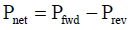
Where Pnet and d are the net power input to the TEM cell and the distance between a septum and ceiling conductor of the TEM cell, respectively. In the TEM cell that is used in the experiment, d is equal 150 mm. Pnet is calculated by measuring the incident power Pfwd and the reflected power Prev from the TEM cell using a power meter (Anritsu 4803A) in (Figure 11) and using (Equation 16).
 (16)
(16)
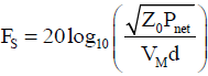
However, the output terminal of the directional coupler and the TEM cell input terminal are connected by coaxial cables, and the coupling factors of the directional coupler also has frequency characteristics. It is necessary to correct the cable loss and the coupling factors of the directional coupler to applying Eq.(16). On the other hand, when the indicated value of the signal voltage sent from the RF output of PD / LD of the OES to the spectrum analyzer (HP 8560E) is VM, the antenna factor Fs is obtained as the following equations according to the definition of the antenna factor (See Equation 1).
 (17)
(17)
 (18)
(18)
The procedure of the OES calibration is as follows:
(1) Set the frequency of the signal generator (Agilent E4438C) and turn on the output.
(2) Measure the incident power Pfwd and the reflected power Prev with the power meter to obtain the net power Pnet.
(3) Measure the RF output voltage VM from the sensor to be calibrated with the spectrum analyzer.
(4) Repeat from (1) to (3).
Since the nominal upper-limit frequency of the TEM cell is 500 MHz, the calibration was performed up to this frequency. The calibration result is shown in (Figure 12). In the figure, the characteristics are disturbed around 2 MHz, but the antenna factor is a constant value at about 66 dB/m more than 200 kHz. The value is almost the same value as the manufacturer's specifications. It was found that the value of the antenna factor below 200 kHz increases (i.e., the sensitivity decreases) as the frequency decreases.

Figure 12. Measurement result of antenna factor for OES.
The OES introduced in the previous section is excellent for a purpose of measuring electromagnetic fields in the vicinity of electrostatic discharges because of its low invasiveness and the flatness of the antenna factor. However, the antenna factor of 66 dB/m cannot be said that highly sensitive because the larger the value of the antenna factor the larger the correction quantity. Therefore, it is not necessarily suitable for measuring a distant electromagnetic field away from the ESD source. This section introduces a newly designed and developed high sensitivity and broadband antenna and describes the results of measuring the VSWR, complex antenna factor, and antenna gain of the antenna. The superiority of this antenna in the far-field measurement of the ESD transient electromagnetic field will be indicated from the result.
A. Folded Rhombic Antenna
The folded rhombic antenna (Okamura antenna) had been developed by Prof. Okamura et. al. in 1950s [11]. This antenna has a wide usable frequency band from 260MHz to 700MHz. Figure 13 shows the top and front views of the antenna. This antenna has a structure in which a diamond-shaped conductor plate is symmetrically bent inward in a curved shape. The tips of the rhombic conductor plate are oriented into a small hole in the center of the rhombus as a balanced feeding. Table 1 shows the dimensions of the two types (type A and type B) that has been investigated by Okamura (See also (Figure 13)) for the dimensions of each part). (Figure 14) shows the measurement results of the real and imaginary parts of the self-impedances of the antenna in the two types shown in (Table 1). In the figure, the real part of the self-impedance of the antennas is about 200 Ω and the imaginary part is about 0 Ω, especially in type A. This result shows the antenna has a broadband performance for UHF frequency band.
| [mm] | D1 | D2 | w | b | h |
|---|---|---|---|---|---|
| Type A | 340 | 235 | 45 | 125 | 340 |
| Type B | 265 | 165 | 35 | 155 | 340 |

Figure 13. Top and front views of folded rhombic antenna.

Figure 14. Frequency response of folded rhombic antennas [11].
B. Folded Long-Hexagon Antenna
To extend the usable upper limit frequency of the folded rhombic antenna to microwave band, we designed an antenna with a new shape based on the half size of the original type-A antenna. In this case, the shape and dimensions were partially changed, and the shape of the antenna element was changed from a rhombus to a long hexagon. (Figure 15) shows the shape and dimensions of a newly designed antenna. (Figure 16) shows photographs of the appearance of the designed antenna. In the figure, the proposed antenna has a structure in which a long hexagonal metal plate is symmetrically folded inward. The dimensions are 230 mm in width, 170 mm in depth, and 145 mm in height, and weighs about 300 grams. The proposed antenna is lighter and more compact than conventional antennas for EMI measurements such as a double-ridged guide horn antenna (DRGHA) that is commercially available. Styrofoam is installed in the center of the folded part of the antenna element to protect its shape. In addition, an electromagnetic absorbing sheet with a thickness of 10 mm was installed inside the antenna to reduce small fluctuations of antenna gain response.

Figure 15. Shape and dimensions of folded long-hexagon antenna.

Figure 16. Front and top views of folded long-hexagon antenna.
The complex antenna factors and antenna gains of the proposed antennas are obtained by the 3-antenna method of which principle is explained in Section II B. The transmitting S-parameters were measured by a VNA (Agilent E8762B). An antenna height is set to 1.2 m from the top of EM absorbers installed on the ground plane in an anechoic room. A height of the EM absorber is about 80 cm. The distance between the transmitting and receiving antennas was set to 3 m in the measurement.
Figure 17 shows the measured voltage standing wave ratio (VSWR) of the proposed antennas. In the figure, #1, #2, and #3 denote the antenna numbers. This value indicates a degree of power reflection from the antenna, and the closer the value is to 1, the smaller the reflected power when power is applied to the antenna. The small vibration in the characteristics shown in the figure may be due to a defect in the calibration of the VNA. Taking the median value of this vibration, the VSWR of the antenna is about 2 or less from 500 MHz to 20 GHz.

Figure 17. Measurement result of VSWR.
(Figure 18) shows the measurement results of the amplitude of the complex antenna factors. In the figure, #1, #2, and #3 denote the antenna numbers. In the result, the amplitudes of the complex antenna factors are in the range of 20 dB/m to 40 dB/m, and has a logarithmic linear characteristic more than 2 GHz. (Figure 19) shows the measurement result of the phase of the complex antenna factor. In the figure, the proposed antenna has an extremely small phase deviation of ± 5 ° more than 1.3 GHz. Therefore, it can be expected that the electromagnetic field due to an ESD phenomena in the far-field region can be measured by using the proposed antenna with almost no distortion of the impulse waveforms.

Figure 18. Measurement result of complex antenna factor in amplitude.

Figure 19. Measurement result of complex antenna factor in phase.
(Figure 20) shows the result of calculating the absolute gains from the complex antenna factors Fc using (Equation 19).

Figure 20. Measurement result of absolute antenna gain.
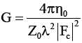 (19)
(19)
In the figure, the absolute gains have the characteristics of monotonically increasing from 500 MHz to 20 GHz and is from 0 dBi (500 MHz) to a maximum of 15 dBi (20 GHz). This frequency characteristic suggests that the newly developed antenna can be used in the frequency band exceeding 20 GHz. On the other hand, the antenna gain of the commercially available DRGHA does not exceed 12 dBi, and we can see the gain drops rapidly at frequencies above 18 GHz. Therefore, the developed antenna is not only suitable for measuring transient electromagnetic fields such as an ESD field, but also suitable as an antenna for EMI measurements.
In this paper, we introduced measurement techniques of the wideband transient electromagnetic field generated by ESD phenomenon. By converting the waveform observed by an oscilloscope into the frequency domain using the discrete Fourier transform, removing the characteristics of measuring apparatus such as the broadband amplifier measured by the S-parameters, and applying the complex antenna factor of the antenna / sensor. It was shown that these data were converted using the inverse Fourier transform, then the real waveforms of the electromagnetic field were obtained. We also introduced antenna / sensor calibration methods specialized for the far field and the near field, and examples of their characteristics. In particular, the usefulness of a broadband folded long-hexagon antenna for far-field measurements was shown.
This research/development includes the results carried out by the Ministry of Internal Affairs and Communications "Research and Development for Expansion of Radio Resources (JPJ000254)".