Role of Spatial Variability in the Service Life Prediction of RC Bridges Affected by Corrosion

Omran M. Kenshel^1*, Alan J. O’Connor², Mohamed F. Suleiman¹ and Fauzi E. Jarushi^1
*Correspondence: Omran M. Kenshel, Department of Civil Engineering, Faculty of Engineering, University of Tripoli, Libya, Tel: +218-924938411, Email:

Keywords

Service life prediction • Chloride ingress • Reinforcement corrosion • Monte Carlo simulation • Spatial variability.

Introduction

For Reinforced Concrete (RC) bridge structures located in marine environments, different deterioration mechanisms have been recognized, e.g. carbonation-induced corrosion, freeze/thaw, alkali-silica reaction, sulphate attack, etc. The majority of RC bridge structures in marine environments, however, deteriorate mainly due chloride-induced corrosion [1]. Furthermore, for corrosion affected RC bridge structures in marine environments, repairing costs due to concrete cracking and spalling exceed those from other forms of deterioration by a substantial margin [2]. It is, therefore, RC bridge structures in marine environments deteriorating due to chloride-induced corrosion which will be the focus of this paper. Many models have been proposed by various researchers to describe the deterioration process of RC structures exposed to chloride induced corrosion. These models often used by researchers in a probabilistic framework to allow for the inherent variability of the model parameters to be considered. This can be done by describing each model parameter within the deterioration model as a random variable characterized by its Probability Density Function (PDF). However, by modeling each parameter as a random variable with a specified PDF mean (μ) and standard deviation (σ), the Spatial Variability (SV), i.e. the fluctuation of properties in space, of the model parameters is ignored. It may be accepted that some model parameters, such as the yield strength of the reinforcing steel, would exhibit very little SV due to the high quality control that is implemented by the manufacturer. However, many material and geometrical properties, e.g. cover depth, concrete compressive strength, are expected to show considerable SV due to the effect of environmental conditions and the inconsistency of the workmanship. It is tabulated that neglecting such sources of uncertainty will have some impact on the evaluated safety and the whole life durability performance of the structure. Investigating the magnitude of this impact on the safety profile of the structure has been the prime objective of this paper.

Research Methodology

Formulation of service life models

The material deterioration models often described in the literature in the context of structure service life modelling where each stage of the deterioration process is quantified in terms of time and the sum of these times makes the total service life. For RC structures, it is postulated that during the hydration of cement a highly alkaline pore solution (pH between 13 and 13.8), principally of sodium and potassium hydroxides, is gained [3]. In this alkaline environment a protective oxide layer, a few nanometers thick, is formed on the reinforcing steel bar embedded in concrete. In spite of its attested protective property against mechanical damage of the steel surface, the formed layer can be destroyed by carbonation of concrete or by the presence of chloride ions leading to the depassivation of the reinforcing steel. This stage of the service life of RC structures affected by corrosion-induced deterioration is referred to as the Initiation stage, Figure 1. The second distinguished service life stage begins when the steel reinforcement is depassivated and the corrosion process begins its activity and finishes when an undesired limit state is reached prompting a rehabilitation action to be taken. This stage is referred to as the Propagation Stage.

The initiation stage

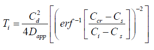
The first step towards a practical quantification of the service life of an RC structure exposed to a chloride rich environment is to predict the time it takes for the chloride ions to penetrate the concrete cover and reach the reinforcement in enough quantity to depassivate the reinforcement, and hence initiate corrosion. Traditionally, the time for chloride ions to penetrate through the concrete cover from the surface and reach a critical (threshold) value Ccr at the level of reinforcement, has been modelled using an expression derived from Fick’s 2^nd law of diffusion.

(1)

Where T_i is time to corrosion initiation (years); D_app is the diffusion coefficient in (mm²/year); Cs is the surface chloride content, C_i is the initial chloride content and C_cr is the critical chloride content. C_s, C_i, and C_cr are in (Cl% per mass of cement or concrete) and C_d is the reinforcement cover depth in (mm). D_app, C_s and C_i, are often determined by fitting data of chloride concentration obtained from chemical analysis of concrete dust samples taken across the depth of the structure to Fick’s 2^nd law of diffusion. In this paper the data on the aforementioned two parameters were obtained from the analysis of 45 concrete cores collected from Ferrycarrig Bridge located on the south west of Ireland [4].

The propagation stage

As the propagation stage starts, the cross-sectional area of longitudinal reinforcement of the RC beam, which provides its flexural capacity, will be reduced due to the ongoing corrosion activity, leading to rupture at the critical cross-section of the RC beam. Similarly, the shear links, which provide the beam with a substantial proportion of its shear capacity, lose some of their cross-sectional area as corrosion progresses. Consequently, the structural safety of the beam will be reduced over time. In this paper, the structural safety of the considered beam girder is determined with respect to the flexural and the shear strengths although other effects (e.g. torsion, fatigue, etc.) can equally be considered.

Flexure resistance models

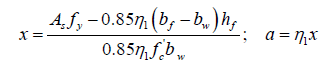
In AASHTO-LRFD, the computation of the flexural capacity is based on the Whitney’s rectangular approximation of the parabolic stress distribution showed in Figure 2(a) [5,6]. In order to determine the flexure capacity of an RC T-beam section, two cases have to be considered, case (1) where a≤h_f and case (2); where a>h_f, (h_f is the flange thickness of the T-beam), To determine if a≤h_f, the distance x shown in Figure 2(a) (the distance from the extreme compression fiber to the neutral axis NA) must be found according to (3) (Figure 2).

(2)

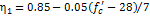
While values for the parameter η1 are given in Table 1, all other parameters are as defined in Table 1 [7].

The computation for the beam flexure capacity at any time (t) of a T-section can be carried out for the two cases (assuming only the reinforcement crosssectional area is reducing with time due to the effect of corrosion, no bond loss or anchorage slip is considered as follows:

Case (1): a ≤ h_f, Figure 2(b).

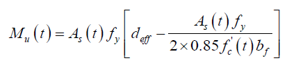(3)

Case (2): a > h_f, Figure 2(c).

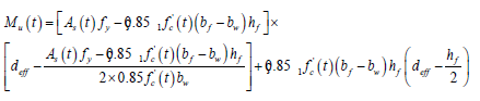(4)

Where all variables involved in the formulation of (3) & (4) are defined in Figure 2 and Tables 1 and 2.

Shear resistance model

Similarly, the time-dependent ultimate shear resistance of the beam at any given section is calculated by simply combining the contributions of concrete and shear links to the shear resistance of the section provided by AASHTOLRFD as follows [7]:

V_u = V_c + V_s (5)

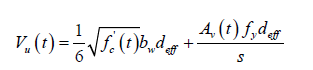(6)

Where all parameters in (6) & (7) have been defined in Table 2. Equation (7) was derived from an expression that is based on the variable-angle truss model for a uniformly loaded beam in which the beam is treated as a truss with a diagonal crack in which the local stresses at the crack (indicated in Figure 3) must be in equilibrium. In the original derivation of (7) the vertical forces acting on the diagonally cracked section were set to be in equilibrium, the distance between the tension and the compression reinforcement, d_v, were approximated by d_eff and the angle φ was taken as φ=45° whereas V_ci was experimentally related to fc’ so that V_ci=1/6√ fc’ (MPa).

Modelling the concrete compressive strength

In design, the characteristic strength (f_ck’), rather than the mean strength, is used (i.e. f_c’= f_ck’ in all previous code-provided equations). This strength is defined as the level below which only a small proportion (usually 5%) of all the results are likely to fall [8]. When concrete is ordered, it is a concrete with some specified characteristic strength that will be asked for. To ensure this, the producer has to provide a concrete with an average strength that is well above the specified characteristic strength. The amount by which the average exceeds the characteristic value depends on the effectiveness of the producer’s control methods. Eurocode 2 (EC2) relates the concrete mean cylinder compressive strength to the specified characteristic strength for concrete up to 50 MPa as follows:

f’_cyl = f’_ck +8(MPa) (7)

Based on worker performance survey data, Stewart performed a probabilistic analysis in which he then proposed that the actual concrete compressive strength mean (μ) and coefficient of variation (COV) of the assessed structure may be related to the compressive strengths obtained from the standard test cylinders, which are cured and compacted under standard conditions, as follow [9]:

μ( f’_c ) = μ( k_w )+μ( f’_cyl ) (8)

 

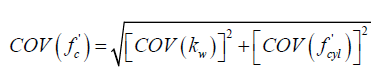
(9)

Where (k_w) is a workmanship reduction factor that takes into account the influence of workmanship quality (i.e. curing and compaction) on the actual structure concrete compressive strength and its values can be obtained from Table 3. The analysis carried out in this paper assumed ‘Fair’ worker performance with ‘minimum 7 days curing time’.

To allow for the influence of time-dependent increase in concrete compressive strength to be considered in the current analysis, the parameter f_c’, which represents the 28 concrete compressive strength in (4), (5) and (6) can be replaced by a time-dependent compressive strength f_c’(t). The following expression proposed by ACI 209 has been used in reliability based assessment of corroding structures and therefore it was used here to model the evolution of concrete compressive strength with time 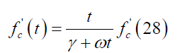[10].

(10)

Where t is the time elapsed since the beam construction in days, γ=4.0 and ω=0.85 for moist cured Ordinary Portland Cement (OPC).

Model error of the resistance models

Based on a study conducted on 1146 RC beams aimed at comparing experimental shear strengths with those obtained from predictive models provided by a number of national standards and codes (e.g. ACI, AASHTO, BS 8110 and EC2), Somo and Hong found that predicting the shear capacity of a RC beam with shear links using (7) may lead to underestimation of the shear capacity of the RC beam [11-15]. They recommended a model error (bias factor) with a mean value of 1.3 and a coefficient of variation that is larger than 0.3 to account for the uncertainty associated with the use of the predictive model proposed by codes and standards used for estimation of the shear capacity. No similar experimental-based study has been reported in the literature with regard to the flexure capacity. However, based on simulation of moment-curvature relationship performed by Tabsh and Nowak a mean model error of 1.14 and a coefficient of variation of 0.13 were proposed to account for the uncertainty associated with the flexure resistance model determined according to AASHTO-LRFD [16].

Materials deterioration models

Models describing the loss in the flexure and shear capacities over time due to the chloride-induced corrosion will be covered in this section. These models are vital for formulating the LS functions which will be employed to estimate the Probability of Failure (P_f) and hence the Reliability Index (β). Reliability Index (β) is an indication of the performance of the structural safety and is related to the (P_f) through the following expression [17]:

(11)

Where Φ(.) is the standard normal distribution function.

Before proceeding to describe the models used for determination of the residual flexure and shear capacities of the RC beam due to general and pitting corrosion, the resistance models will first be presented.

Modelling loss of reinforcement

In this paper two forms of corrosion mechanisms were considered for the reduction in the reinforcement cross-sectional area. These are the General corrosion and the Pitting (localized) corrosion. General corrosion affects the reinforcement by causing a uniform loss of its cross-sectional area. Pitting corrosion, in contrast to general corrosion, concentrates over small areas of the reinforcement. The calculation of the residual cross-sectional area of the reinforcement due to any of the two types of corrosion will be explained here.

Due to general corrosion

If the corrosion is assumed to be of a uniform type, often referred to as ‘General corrosion’, Figure 4, the loss of reinforcement diameter can be described by the use of Faraday’s law of electrochemical equivalence [18]. Faraday’s law indicates that a constant corrosion rate of 1.0 μA/cm² corresponds to a uniform metal loss of bar diameter of 0.0232 mm per year (or 1.0 μA/cm²=11.6 μm/year metal loss of the bar radial). If the corrosion rate is assumed to be constant over time, then the remaining cross-sectional area of corroding main reinforcement after t-years A_s(t) can thus be estimated as:

(12)

p_max(t) = 0.0116i_corr ( t - T_i ) R (13)

Due to pitting corrosion

Pitting (localized) corrosion is very intense form of corrosion in which a small area over the reinforcement length may suffer much greater loss of section than the rest of the reinforcing bar. For that reason, the measurements of the corrosion rate (i_corr) cannot be directly translated into the loss of crosssectional area of the corroding bar in the same way indicated by (13). According to Gonzalez et al. the maximum penetration depth caused by pitting corrosion (P_max) can be 4 to 8 times of that caused by general corrosion [19]. This conclusion was derived from results obtained from testes made on specimens of 125 mm long and have a bar diameter of 8 mm. The corrosion rate icorr for general corrosion can be related to P_max at any time t via the ratio R=P_max/P_av, where P_av is the average penetration depth expected from general corrosion (P_av= ΔD/2). Therefore, the maximum pitting depth in (mm) at any time may be estimated as follows [19]:

p_max(t) = 0.0116i_corr ( t - T_i ) R (14)

Where Ti is the time to corrosion initiation (years), n_b is the total number reinforcing bars and D_o is the original bar diameter and ΔD(t) is the reduction of bar diameter at time, t (Figure 4).

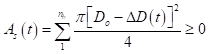
In order to be able to use values of P_max(t) to estimate the loss of crosssectional area of the reinforcing bar due to pitting corrosion, hence estimating the residual cross-sectional area of the reinforcement, an assumption regarding the shape of the pit has to be employed. Few such configuration has been provided by other researchers, e.g. Rodriguez et al. Figure 5(a) and Val and Melchers, Figure 5(b). As shown by Figure 5, Rodriguez et al. configuration seems very conservative as a large proportion of the cross-sectional area of the bar is discarded as a result of the simplified approach. On the other hand, Val and Melchers configuration tends to calculate the exact area of the pit. For that reason, the assumption made by the later researchers was adopted for the analysis in this paper [20,21].

The residual cross-sectional area of a single corroding bar at any time t can be calculated as follows:

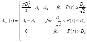(15)

Where:

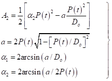(16)

Finally, the remaining total cross-sectional area of the reinforcement subjected to pitting corrosion, after (t-T_i) years of active corrosion, As(t) can be estimated as follows:

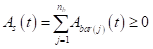(17)

Where n_b is the total number of longitudinal reinforcement bars.

Modelling the corrosion rate (i_corr)

As can be seen from the relations given in the previous section, the corrosion rate is a key parameter for determining the residual cross-sectional area of both, the flexure and shear reinforcements and hence the residual capacity of the deteriorating structural member. Usually i_corr is governed by the availability of water and oxygen at the steel concrete interface, the concrete quality, cover depth, temperature and humidity [22]. Considering the importance of icorr as the key parameter which can influence the rate by which the reinforcements cross-sectional area is reduced, several attempts have been made to predict the corrosion rate where field data on the parameter are not available. In this regard, for a typical environment of an ambient relative humidity of 75% and temperature of 20C°, Vu and Stewart suggested an empirical formula for the estimation of corrosion rate at the start of the corrosion activity i_corr(1). The proposed model relates the corrosion rate to water/cement ratio (wc) and the cover depth (C_d) as follows [22]:

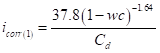(18)

In a real case assessment, it is highly desirable that values of i_corr are obtained from site specific measurements taken from the structure that is under investigation. However, in many cases, as in this paper, field data on i_corr measurements may not be available, therefore, an empirical model such as that proposed above can be used to estimate the i_corr for a given structure with a set of environmental conditions and material properties. According to Duprat, results obtained from (19) found to be in agreement with corrosion rate measurements obtained from experiments performed by Gonzales et al. (1995) and with the average corrosion rate field measurements suggested by other researchers [23]. Therefore, in this paper, the empirical corrosion rate model proposed above by Vu and Stewart was used to produce values of i_corr.

Meanwhile, there is strong evidence to suggest that corrosion rate reduces over time as suggested by Liu and Weyers due to the formation of rust products which slow down the diffusion of irons away from the steel surface [24]. To account for the time-dependent reduction of the corrosion rate, Vu and Stewart suggested that corrosion rate values obtained from (19) can be modified so that the corrosion rate time-dependent can be obtained as follows [23]:

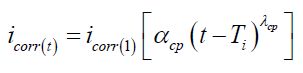(19)

Where (t-T_i )≥1.0 year, α_cp and λ_cp are constants for describing the reduction of the corrosion rate with time their proposed values are 0.85 and -0.3 respectively. The corrosion rate model described above has been used by several other researchers to predict the life time safety performance of RC structures [23,25,26].

In a real case assessment, it is highly desirable that values of icorr are obtained from investigated structure. However, in many cases, as in this research, field data on i_corr measurements may not be available, therefore, (19) and (20) maybe used to estimate the i_corr for a given structure with a set of environmental conditions and material properties. In this paper, Vu and Stewart (2000) corrosion rate model was used to produce values of i_corr that correlate well with the concrete quality and the chosen cover depth used for the considered structure. Care will have to be taken when employing (19) and (20) so that produced values of i_corr correspond well with the commonly field measured i_corr data reported by the literature.

Spatial variability modelling

In a classical reliability analysis problem, material and geometrical properties within a structural component was often treated as homogeneous (perfectly correlated) or randomly distributed (spatially uncorrelated) [21,23,27,28]. However, in reality such properties usually exhibit some limited spatial correlation, Figure 6. That is to say, two samples taken very close to each other can have highly correlated properties and as the distance separating the two samples is increased, the correlation of their properties will decrease. Once the essential characteristics of such fluctuation are obtained, the uncertainty associated with spatial variability of the property of interest (i.e. concrete impressive strength, cover depth, etc.) can be accounted for by dividing the structure surface into number of small elements [29]. Each element will be assigned a value for each of the modelled properties so that the correlation between different elements will depend on the distance separating them. The size of each element (hence the number elements) will depend on the intensity of the spatial fluctuation of the modelled property.

To demonstrate how SV modeling is carried out, a hypothetical RC beam was used in this study, details of the RC beam adopted here were taken from Enright and Frangopol [30]. The RC beam is a part of a highway bridge located near Pueblo, Colorado and is designated as ‘Colorado Highway Bridge L-18- BG’. The bridge consists of three 9.1 m simply supported spans where each span has five girders @ 2.6 m centers. The cross-section of the beam girder is shown in Figure 7(a). In this paper, the considered beam girder was assumed to be subjected to chloride ions penetration from all three exposed surfaces as indicated in Figure 7(b). As indicated earlier, in SV modeling, material and geometrical properties are considered not to be perfectly correlated (i.e. spatially constant) within a structure or a component, but rather vary across the structure with some limited field correlation. For this spatial variation to be considered, the structure needs to be divided into a number of small square/ rectangular elements so values for the random variables can be assigned for each element with correlation between the elements taken into account during the random variables generation process.

Structural discretization

In the beam girder under consideration, for the two vertical sides of the beam, a Two-Dimensional SV model that would take into account the fluctuation of the random variables in both directions can be used. If the fluctuation of random variables in one direction of the beam (e.g. the transverse direction) can be neglected compared with the longitudinal direction, a simple One-Dimensional SV model can be applied. In the current case, in the One-Dimensional SV model, the beam is discretized into strips (rectangular elements) of a width Δ_x (m) and a height that is equal to height of the beam web (h_w) as showed in Figure 8(a). In the Two-Dimensional RF model the vertical faces of the beam were divided into multiple equal segments with a vertical size Δ_y = h_w/k_y (m) where k_y is the number of SV elements specified for the vertical direction, Figure 8(b). The same meshing principle could be applied to the bottom face of the beam; however, due to the relatively smaller width of the beam bottom (b_w=0.4 m) as compared with the length of the beam (9.6 m), only One-Dimensional meshing model was considered for the bottom face Figure 8(c). Determining the size of the SV elements will be discussed in the following section.

Size of the VS elements

The size of the discretized SV element to be chosen depends on the parameter θ of the random variable of interest and the correlation coefficients between the two neighboring elements calculated using the autocorrelation function. If the size of the SV element is too large, this implies that the random variable is constant within each element which may results in underestimation of the effect of spatial variability of the random variable particularly when the value of θ is too small relative to the SV element size. On the other hand, a small element size leads to the generation of a very fine mesh that causes the random variables in elements close to each other to have high correlation with each other resulting in numerical difficulties in the decomposition of the correlation coefficient matrix. Interested readers are referred to reference for more details on this issue [31]. Therefore, the SV element size has to be chosen in such a way to avoid high correlations among the random variables specified for neighboring elements. The available literature has recommended that the element size should be between θ/4 and θ/2. A sensitivity analysis was performed by the first author to define the optimal element size for the beam example under consideration. The optimal element size in this case was found to be ∆_x= 0.31 m for One-dimensional SV model which corresponds to using 31 elements for the beam.

The autocorrelation function

The autocorrelation function ρ(τ) is a mathematical expression needed to specify the correlation behavior between observations as a function of the separating distance (i.e. between any two neighboring SV elements separated by distance, τ). The role of the autocorrelation function in SV modeling is explained in details by the author in [31]. There are several autocorrelation functions have been proposed in the literature to choose from [32]. To date, no specific autocorrelation function has been favored for the type of analysis that is similar to the one carried out in this study. However, the Square Exponential autocorrelation function, is the most frequently used by researchers in field of RC corrosion [29,33,34] and therefore was used in the current paper to generate the correlated data for each SV element. The Two-Dimensional form of the Square Exponential autocorrelation function is expressed as follows:

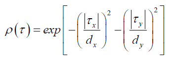(20)

Where d_x and d_y are the model parameters (correlation lengths) for a Two- Dimensional SV in x and y direction respectively which is related to the scale of the fluctuation, θ, through the relation θ=√πd, and τ_x=x(j+1)-x_j, τ_y=y(j+1)- y_j are the distances between center of elements j and j+1 in x and y directions respectively. If a One-Dimensional SV model is considered the y component is neglected.

It can be observed from (21) that the degree of correlation between the SV elements is dependent upon two main parameters; the correlation length (d), hence θ, and the distance (τ) which is directly dependent on the element size ∆x and ∆y. In order to obtain an appropriate d value for a SV variable (i.e. a random variable that is also a spatially variable), data sets consisting of sample measurements taken at frequent distances are needed. In practice, such measurements are rarely taken at frequent distances; consequently, data on d are scarce and usually assumed based on engineering judgment. However, in the current study values for the parameter d for two key deteriorating variables, namely Cs and Dapp, were obtained following extensive experimental and numerical/statistical analysis carried by the author [31]. The values of the parameter d were determined for both variables by performing spatial correlation analysis on the data collected from the ageing RC Ferrycarrig Bridge [4].

Based on the spatial correlation analysis performed by the first author in, values of d (hence θ) were found to be as indicated in Table 4 [35]. Due to the positive correlation between D_app and other concrete properties such as f_c’, wc and i_corr (1), it was reasonable to assume that these later variables have similar fluctuation properties as that of their associated variable, D_app. Therefore, all variables which are dependent on or related to D_app were assumed to have the same θ value as that found for D_app. For all other SV variables, values of θ that have been used by other researchers in the field [29,33] indicated in Table 4 were used.

Generation of random variables for SV modelling

When a simulation technique is used, the non-correlated standard Gaussian field is obtained through a procedure consisting of two steps:

1) Random numbers uniformly distributed between 0 and 1 are generated and stored in a vector U. (Note that the number of elements of vector U is equal to the number of SV elements).

2) In the second step, the non-correlated standard Gaussian field is obtained with:

Y = φ^-1(U) (21)

Where Φ(.) is the standard normal distribution function. The randomly generated variables (vector Y) are non-correlated; therefore, they need to be transformed in such a way so that the resulting vector possesses a certain correlation between its elements. The procedure for generating spatially correlated random variables, which is summarized in Figure 9, is described in full details in [35].

Reliability model (Safety profile)

To illustrate how SV is expected to influence the safety profile (i.e. the life time safety deterioration) of the RC beam under consideration, two cases were considered. In the first case, the deterioration properties were assumed to be constant along the beam which is equivalent to the state of Perfect Spatial Correlation (i.e. d ≈ ∞). This is also similar to the conventional structural reliability analysis which tends to evaluate the failure probability (P_f) of the Limit State (LS) only at sections within the structure where the highest load effect is expected. For example, for a simply supported beam, these sections are the mid-span for the flexure LS and the end support for the shear LS. In this way, SV is ignored and P_f is determined based on evaluating the LS functions at a single SV element located at what deemed to be the critical section.

In the second case, the SV of the deteriorating properties along the beam was considered, this is the state of Spatial Correlation. Each SV element was considered as an individual component and its individual P_f was used to form a system reliability problem for the whole beam. In this case, the governing LS was not always violated at sections (i.e. center of SV element) within the structure where the highest load effect is induced as mentioned earlier. Other sections along the beam may experience the LS violation first as will be shown later.

Formulation of the (LS) function

In order to calculate the annual failure probabilities (Pf) of the beam under consideration and hence its safety profile, a limit state function (LS), which depends on a set of basic random variables, in terms of each failure mode needs to be formulated and evaluated at the center of each SV element. Two LS functions were considered for the beam problem at hand; the Flexure and the Shear limit states.

Flexure failure LS: The corresponding LS function for beam failure in flexure at any given time (t) during the service life of the beam GM(t) is as follows:

G_M (t) ≤ 0 ; G_M(t) = M_u(t) - M_b(t) (22)

Where M_u(t) is the ultimate bending moment capacity of the RC section at time t (years) and can be calculated according to the relevant design code. In this paper M_u(t) estimated from (4) or (5). M_b(t) is the induced bending moment at the same section at the same year and it will be estimated later in the upcoming section.

Shear failure LS: The corresponding LS function for beam failure in shear at any given time (t) during the service life of the beam G_V(t) is as follows:

G_V(t) ≤ 0 ; G_V(t) = V_u(t) -V_b(t) (23)

Where V_u(t) is the ultimate shear capacity of the RC section at time t (years) and can be calculated according to the relevant design code. In this paper V_u(t) is estimated from (6) and (7). V_b(t) is the induced shear force at the same section (element) at the same year (t) and will be estimated from the following section.

Load modelling

In previous studies, the load models used to assess the load carrying capacity of corroding structures were either oversimplified or estimated from conservative standards or codes of practices and not from actual traffic data. In this paper, the load model used was based on a realistic site-specific load data acquired by the second author using Weigh in Motion (WIM) technique [36]. In the process, a desired amount of traffic data is generated from the available WIM record. The resulting load effect data, i.e. bending moment and shear force, is obtained using influence lines procedure. The calculated bending moments and shear forces are then fitted to an Extreme Value (EV) distribution such as Gumbel Type I distribution or Weibull distribution using probability paper. The selection of the appropriate distribution is based upon linearity of the data plotted. In the present study, Monte Carlo (MC) simulation, a method to be discussed in the following section, was carried out to generate 4 weeks of traffic data, based on the information provided by the 7 days WIM record provided in [36]. The data obtained from the simulation were extrapolated to determine the extreme load effects for a desired reference period of 100 years (i.e. the bridge design life). For further details on this subject the reader is referred to [4]. The maximum load effect results for different return periods for moment and shear were summarized in Table 5.

Values in this table represents M_b(t) and V_b(t) were used for the evaluation of LS functions expressed in (21) and (22) depends on the remaining service life (reference period) of the structure under consideration. In this paper, the beam girder was evaluated for 100 years (i.e. the expected service life of nowadays bridges), therefor values of M_b=2062 kN.m and V_b=453 kN were used.

Girder distribution factors (GDF)

Having determined the maximum load effect for the desired return period, the value of the moment/shear obtained from the extrapolation does not represent the maximum bending moment/shear acting on a single RC beam girder; this value thus far represents the predicted maximum moment/shear induced by the presence of the heaviest trucks on the bridge deck as a whole in the longitudinal direction. The proportion of this value that is resisted by a single RC beam girder can be determined by multiplying the obtained value by a specified GDF. In the current study, GDFs for the interior girders were calculated in accordance with formulas provided by AASHTO-LRFD [5]. For the beam girder example under consideration, the mean values for the GDFs were calculated for the two loading cases (multiple and a single lane loading) and the result are as presented in the following table (Table 6).

Based on field testing and finite element analysis, Eom and Nowak suggested that for simply supported bridges the AASHTO-LRFD GDFs for one lane loading is more realistic for estimating the design load effect [37,38]. The uncertainty in the GDFs may be expressed in terms of the model error (bias factor). For GDFs based on simplified code methods such as that provided by AASHTO-LRFD, a normally distributed bias factor with a mean value of 0.93 and coefficient of variation of 0.12 were reported in the literature for the case of bending [38]. No such information was reported with regard to GDF for shear, therefore, the bias factor’s mean and coefficient variation for the bending moment GDF’s are assumed to be valid for the case of shear.

Monte Carlo (MC) simulation

MC simulation is a technique which involves random sampling of variables to artificially produce a large number of experiments (or solutions of an algebraic equation) and observe the results. In the context of structural reliability analysis, this means, each basic random variable is randomly sampled from a specified PDF (Normal, Lognormal, Gumbel, etc.). The LS function G(X) is then checked; if the LS is violated (i.e. G(X)≤0), then the system has failed. The experiment is repeated many times, each time with a randomly chosen vector of values for the involved basic random variables. If N trials are performed, the probability of failure is approximated by:

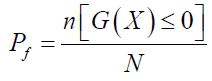(24)

Where the expression n[G(X)≤0] denotes the number of trials n for which G(X)≤0.

The ability of (25) to accurately estimate Pf depends on the number of simulations N. Theoretically, the estimated Pf will reach the true value as N→∞. However, the number of simulations N that can be performed will be limited by the speed of the computer processor that is used. It has been reported (e.g. by Haldar and Mahadevan, 2000) that the Pf obtained using MC simulation is almost the same as that obtained from other analytical method such as the First Order Reliability Method (FORM) when the number of simulation is relatively large [39]. One has to accept that there should be a ‘Trade-off’ between the accuracy desired and the time it takes for the computational problem to be solved.

Calculation of the reliability index (β)

Having defined the individual LS functions and assigned the probability distribution to the set of basic random variables and the correlation coefficients between the SV elements, the failure probability for each element with respect to each failure mode can be determined for each year of the structure service life. It has to be noted that when calculating Pf for each period over the service life of the structure, the discretized periods have to be long enough for the correlation between periods to be negligible [23]. For example, Durprat mentioned that for an industrial warehouse loading, the length of independent periods can be estimated at 2 years. Structural assessments of bridges are often based on a limited reference period of 2-5 years and after the end of this period the bridge is normally re-assessed as its structural capacity is likely to change [22]. Thus, it would be more logical and appropriate to compare probabilities of failure for relatively short reference periods. However, too short discretized periods, i.e. one year long, can result in a very long computational time. Therefore, in the present study, due to the lack of reliable data on the correlation between incremental periods, and for the sake of simplicity, the probability of failure will be assumed independent for each incremental time period of 5 years which is within the figures indicated by Vu and Stewart [22]. The procedure followed in this study to calculate the time-dependent reliability (Safety Profile) of the beam girder under investigation as follows:

For a series reliability system consists of (k) SV elements, the critical limit state occurs when the actual load effects exceed the resistance at the center of any element. The critical moment and shear limit state for a One-Dimensional RF model consisting of k elements at any year (ti) can be expressed as follows:

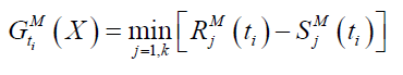(25)

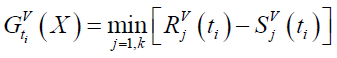(26)

Where and are the flexure and shear LS functions respectively and are the distribution for moment and shear resistance respectively, for element j evaluated at its center at time ti, and are the corresponding load effects at the centre of the same SV element due to the load acting at the same time ti.

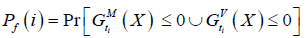
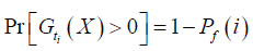
The annual probability of failure of the beam in terms of bending moment (flexure) or in terms of shear can be computed respectively as follows:

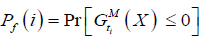(27)

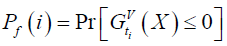(28)

The total annual probability of failure of the beam then can be calculated by combining the probability of failure of the beam in moment and in shear.

(29)

In general, and as indicated by Stewart (2004), if it is assumed that (m) load events Sj occur within the time interval (0, T) at times where i=1,2,3,… ..,m, the cumulative probability of failure any time during the time interval from 0 to T for (m) events is [40]:

(30)

Where:

(31)

If the failure events are assumed independent events, then (30) can be approximated by:

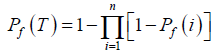(32)

Where P_f (i) is obtained from (29).

The reliability of the structure is then assessed by using the conditional probability of failure which integrates the survival period of the structure prior to the time at which the reliability is estimated [22,23]. To calculate the conditional probability that the beam will fail in t subsequent years given that it has survived T earlier years, the following expression can be used:

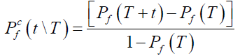(33)

Where P_f (T+t) and P_f (T) are calculated using (30).

Finally, the probability of failure can then be translated into the Reliability Index (β) through the relationship given in (11).

Target reliability (β_T)

In performing a structural safety or reliability assessment the computed reliability index is compared to a target value (β_T), for the considered limit state, and consequence, to determine compliance or violation. Table 7 presents acceptable β_T values as specified by the Eurocode (EN1990-2002). More information on the reliability classes specified by the Eurocode are available in the cited literature.

Important Assumptions

• The random variables are considered constant for a single SV element and each random variable is represented by a value that is evaluated at the center of that element; this implies that when corrosion is initiated in a SV element all reinforcing bars in the same layer in that element are assumed to start corroding at the same time.

• The maximum pitting depths for each bar (or shear link) or for different bars within an element are treated as statistically independent (uncorrelated). This is because of the lack of knowledge on statistical correlation between the corrosion pits.

• After corrosion-induced concrete cracking has taken place, the beam section is still assumed to be physically sound when evaluating the section moment and shear capacities, and only corrosioninduced reduction of the reinforcement cross-sectional area is taken into account. In addition, bond strength between concrete and reinforcement are assumed not to be affected by corrosion; therefore, (4), (5) and (6) were used throughout the lifetime of the beam to estimate flexure and shear capacities.

• If a random variable is assumed to be also SV, all variables which depend on that variable was also treated as a SV. For example, (w_c) and (D_app) are dependent variables on (f_c’), therefore, they are also SV.

• Although several mechanisms exist, chlorides penetration through the concrete cover in the current case was assumed to happen solely due to diffusion. Furthermore, the presence of cracks (e.g. due to load-induced stresses, shrinkage or corrosion product expansion) of a size larger than 0.3mm, may expose the reinforcement to the direct influence of the environment. While it is recognized, this situation has not been considered in the present analysis and its consideration is beyond the scope of this paper.

Results and Discussion

For both failure modes, flexure and shear, and for each of the two forms of corrosion, general and pitting, the annual reliability indices corresponding to the beam annual failure probabilities were calculated for 100 years of the beam service life (in 5 years’ increments).

Influence of pitting corrosion

The influence of pitting corrosion on the safety profile will be discussed in terms of Flexure versus Shear and SV versus NO SV analysis. The results of β(t) indicating Flexure, Shear and Total were produced employing (28), (29) and (30) respectively in (31) and (34).

The reason for not having a complete trend that shows the values for the reliability indices at the very early age is that probability of failure is too small (i.e. Pf ≈0) to be captured by the MC simulation method with a number of iterations that are feasible to performed using commercially available computers. The number of iterations were used to perform the reliability analysis carried out in this study was 1,000,000 (One million) iterations for each incremental year. The entire analysis to produce one safety profile would normally take about 48 hours to complete. Since the focus of this study is to show the relative influence of SV with reference to the NSV scenario and the relative influence of pitting corrosion as compared with the general corrosion case, the 1,000,000 iterations were considered to be sufficient. Furthermore, with this number of simulation iterations, it was possible to produce stable results of the safety profile in which the target reliability can be clearly identified (i.e. β_T=3.8).

Figure 9 indicates that the beam reliability decreases with time. This is due to the reduction of the cross-sectional area of flexure and shear reinforcements. For both cases, general and pitting corrosion, the reduction of the beam reliability over time can be seen to be governed by shear rather than by flexure for both spatial and no spatial analysis. Due to their relatively smaller cover depths as compared to the main flexure reinforcements, shear links are expected to have a shorter T_i period (according to Equation (1)) and a higher value of i_corr (according to Equation (31)). It is therefore expected that shear links are more vulnerable to corrosion attack than the flexure reinforcement. Furthermore, the shear links have a smaller diameter which implies that the percentage loss in the cross-sectional area is more prominent in the case of shear than in the case of flexure. This agrees well with the literature which indicated that the influence of shear failure on the beam reliability increases when higher diameter bars are used for the longitudinal (flexure) reinforcement [41].

Influence of spatial variability

To investigate the influence of considering SV on the safety profile of the beam girder under consideration, results presented in Figure 10 for flexure and shear were re-plotted on a single graph, Figure 11. The first observation can be made from this new figure that SV has no influence on the predicted reliability indices in terms of shear for both cases general and pitting corrosion. This means that the violation of the shear LS was governed by the end support SV element where the induced shear force is expected to be at peak.

The second observation which can be made from Figure 11 is that the influence of SV on the beam reliability in terms of flexure is more evident in the case of pitting corrosion than in the case of general corrosion. For example, after 50 years of service, the inclusion of SV has caused the flexure failure probability predicted in terms of pitting corrosion to increase by 12% over that predicted for the case when SV was not considered (NSV). In the case of general corrosion, the increase in the flexure failure probability was only about 2% for the SV scenario. After 100 years of service, the inclusion of SV has caused the flexure failure probability predicted in terms of pitting corrosion to increase by 40% in comparison with NSV scenario. In the case of general corrosion, this increase was only 7% for the SV scenario. It can be concluded therefore that ignoring SV can lead to overestimation of the beam reliability, more evidently in the case of pitting corrosion, when the reliability of the beam is governed by the flexure mode of failure.

The reason why the influence of SV showed to be more significant in the case of flexure than in the case of shear was attributed to the fact that the critical zone by which the LS experiences violation is wider in the case of flexure than in the case of shear. For example, for the 31 SV elements, there were more elements that are likely to govern the flexure LS than elements which are likely to govern the shear LS. To support this conclusion, a histogram was constructed, Figure 12, to show the frequency of SV elements that has governed the LS for the two failure modes, flexure and shear. Figure 12 shows that the governing LS is not always at the mid-span in the case of flexure or at the end support in the case of shear. However, the figure shows that the mid-span SV element (#16) has governed the LS about 25% of the times. The remaining 75% were shared by all other elements with the element adjacent to the mid-span element have higher proportion than those further away. Meanwhile, in the case of shear, the end support element (#1) has governed the shear LS about 47% of the times. It is clear that the remaining SV elements in this case governed the LS violation fewer times than that in the case of flexure. This explains that why the influence of SV on the reliability of the beam is expected to be more prominent in the case of flexure than in the case of shear.

Figure 12 (reproduced from Figure 11) shows the safety profile predicted in terms of the combined (Total) reliability for general (G) and pitting (P) corrosion with the inclusion of SV and without SV (NSV). The figure indicates that the influence of SV is not significant because (as explained earlier) the combined safety profile in this case is governed by shear rather than flexure. However, it is evident from the figure that pitting corrosion has a stronger effect on the beam reliability than general corrosion. For example, after 50 years of service, the combined reliability of the beam due to pitting corrosion was 1.16 verses 2.35 due to the general corrosion. Thus, it can be said that after 50 years of service, the reduction in the beam reliability due to pitting corrosion is 51% higher than that caused by general corrosion.

If the safety profile is shown to be governed by pitting corrosion, as in the current case, the assumption which neglects the effect of loss of bond between the reinforcement and concrete as a result of excessive cracking or spalling can therefore be justified. For example, since pitting corrosion is localized, it is less likely to cause the disruption of the concrete cover and hence no reduction is expected for the bond strength around the pits [21] (Figure 13).

Time for first repair/maintenance

If the decision on the time to first repair/maintenance is to be made based on Ultimate Limit State (ULS) and its related target reliability as specified by EC2 (i.e. β_T=3.8 for Class CC2), the time to first repair/maintenance was found to be about 25 years after the beam construction in the case of general corrosion, Figure 13. When pitting corrosion was considered, the time to first repair/maintenance would be required after only 11 years of the beam construction. In both cases, the beam has failed to maintain its intended design service life (50 years) by a significant margin. The case is more critical when considering pitting corrosion which is in contrast with what some researchers (e.g. Vu and Stewart, 2000) had postulated [22]. The view of the mentioned researchers was that pitting corrosion would not significantly influence the structural capacity of the corroding structure because it is unlikely that many bars will be affected by pitting. The results presented here, Figure 13, have shown that pitting corrosion is more critical than general corrosion from the safety viewpoint. The results presented here indicate that the time to first repair/maintenance of chloride affected bridge structures should consider the reliability/safety of the structure (i.e. ULS) and should not only rely on the surface (visual) condition (i.e. Serviceability LS). This viewpoint has been shared by other researchers (e.g. Enright and Frangopol, 2000; Onoufriou and Frangopol, 2002) who called for the need that repair/maintenance of deteriorating bridge structures should be based on the safety rather than on the visual condition of the bridge elements [42,43].

Sensitivity analysis

In order to assess the relative importance of each random variable involved in the calculation of the safety profile of the RC beam under consideration, a sensitivity analysis was performed. The sensitivity analysis helps identifying which of the random variables has the greatest influence on the calculated beam reliability. In this paper, the sensitivity of the reliability results (Safety profile) were assessed by recording the change in the reliability indices that corresponds to increasing the mean value (μ) or the value of the standard deviation (σ) of the modelled random variable by 10% [44]. The results of the sensitivity analysis are presented in terms of both general and pitting corrosion and for time periods of t=50 years of beam age, (Figure 14).

It was found, as seen from Figure 14, that the single most important parameter which has the greatest impact on the reliability index is the mean value of C_d. For example, in the case of general corrosion, the mean value of C_d =50 mm was increased by 10%; as a result, changes of +0.49 in the value of β were noted for t=50 years. In the case of pitting corrosion, the corresponding changes in the value of β was +0.32. The figures also indicate that the mean value of the specified concrete compressive strength (fck’), the beam effective depth (d_eff), the Model Error (ME) of the girder distribution factor ME(GDF), ME of the corrosion rate (i_corr), ME of the beam shear resistance (V_u) all have comparatively similar influence in magnitude on the change of β. However, ME(GDF) and ME(i_corr) have an adverse effect on β in contrast with f_ck’, d_eff, and ME(V_u). All other random variables, which have been identified in Table 2, are shown to have minor influence on the predicted reliability for both general and pitting corrosion cases.

It can also be seen from this figure that the reliability indices and hence the safety profile is more sensitive to the change in the mean value of the modelled parameters than to the change in their standard deviation.

Conclusion

In terms of the safety performance, SV was shown to be only important if the beam reliability was governed by the flexure Limit State (LS). In this case, the influence of SV on the reliability of the beam was more evident in the case pitting corrosion than in general corrosion. For the case when the reliability of the structure is to be governed by the shear LS, results showed that SV has no influence. This was explained by demonstrating that the end support RF element has governed the LS 47% of the times as oppose to 25% by the mid-span element in the case of flexure. The reduction of the beam reliability over time was shown to be governed by shear for both spatial and non-spatial analysis. This was attributed to the fact that the shear links are often placed at relatively smaller cover depths, Cd, than the main flexure reinforcements. The shear links are, therefore, expected to have a shorter Ti period and a higher value of i_corr. This indicates that, shear links could have suffered larger cross-sectional/resistance losses than the flexure reinforcement at the same point in time.

For the two types of corrosion studied here, general and pitting corrosion, results showed that pitting corrosion potentially has far more aggressive effect on the reliability of corroding structures than general corrosion. The results also suggested that pitting corrosion affects shear resistance far more severely than it would affect flexure resistance. For example, after 50 years of service, pitting corrosion has caused the shear resistance to reduce by 55% more than that caused by general corrosion. In the case of flexure, no difference between the reductions caused by pitting and general corrosion could be observed. The literature reported that many of today’s deteriorating RC bridge structures, including the bridge taken as an example in this study, deteriorates due to corrosion caused by chloride-contaminated water leaking through the deck joints. This means that an intense form of deterioration can take place in locations where high shear stresses are expected (e.g. beam girders at the supports). Therefore, pitting corrosion at locations of high shear stresses can have a severe impact on the reliability/safety of structures. This had led to conclude that the assessment of the safety of RC beams in corrosive marine environments should consider the effect of pitting corrosion of shear links on shear resistance of the beam, otherwise reliability of the beam may be considerably overestimated. Results presented in this paper has also indicated that if only the general corrosion was considered, the decision of the time to repair/maintenance intervention can be governed by the safety criteria of the structure rather than by the visual condition criteria. Furthermore, if the performance criteria to be considered for the time to first repair/maintenance decision do not take into account pitting corrosion, the predicted time to first maintenance intervention maybe too permissive. These findings strongly point to the necessity of having a bridge management system tool that consider lifetime safety of the structure as a viable indicator for maintenance and repair interventions.

References

1. Mallett, PG. “Repair of concrete bridges: State of the art review” (1994).
2. Zheng, JJ, CQ Li, W Lawanwisut. “Modelling of crack width in concrete structures due to expansion of reinforcement corrosion.” Building Materials and Components (2005).
3. Bertolini, L. “Corrosion of steel in concrete: prevention, diagnosis, repair” Wiley (2004).
4. O’Connor, A and Omran Kenshel. “Experimental evaluation of the scale of fluctuation for spatial variability modelling of chloride induced reinforced concrete corrosion.” ASCE J  Bridge Eng 18 (2013): 3-14.
5. https://store.transportation.org/Common/DownloadContentFiles?id=1648
6. Melchers, Rorber. “Structural reliability: analysis and prediction” 199.
7. Andrade, C and Cruz Alonso. “Corrosion rate monitoring in the laboratory and on-site.” Constr Build Mater 10 (1996): 315-328.
8. https://herbycalvinpascal.files.wordpress.com/2019/04/37.-reinforced-concrete-design.pdf
9. Barker, RM, and Jay Puckett. “Design of highway bridges: based on AASHTO LRFD bridge design specifications” Wiley (1997).
10. Narayanan, RS and AW Beeby. “Introduction to Design for Civil Engineers” Spon Press (2001).
11. Stewart, M. “Concreting Workmanship and its Influence on Serviceability Reliability” ACI Materials Journal 94 (1997): 501-509.
12. Stewart, Mark G. "Time-Dependent Reliability of Existing RC Structures."  J Struct Eng 123 (1997): 896-902.
13. Stewart, MG, and David Rosowsky. “Structural safety and serviceability of concrete bridges subject to corrosion.” J Infrastruct Syst 4 (1998): 146-155.
14. https://www.googleadservices.com/pagead/aclk?sa=L&ai=DChcSEwib562s3PfuAhWQCysKHYFNAHgYABAAGgJzZg&ae=2&ohost=www.google.com&cid=CAASE-Ro40tiwVEqgLVkTvA8SNNC50s&sig=AOD64_0PZDoFwC2ZObuFoOXnmaUsMbrevQ&q&adurl&ved=2ahUKEwjVtJas3PfuAhWCUn0KHRbXBfcQ0Qx6BAgEEAE
15. https://shop.bsigroup.com/ProductDetail/?pid=000000000030161093
16. https://www.googleadservices.com/pagead/aclk?sa=L&ai=DChcSEwig24CA6vfuAhXNBHIKHbCuC8QYABAAGgJzZg&ae=2&ohost=www.google.com&cid=CAASE-RoTTDRp6zv53rCQRaebuGAApc&sig=AOD64_09EinG2lbGmZXPpZ5texAcpaqGxw&q&adurl&ved=2ahUKEwiXovT_6ffuAhWUcn0KHZ5YD_cQ0Qx6BAgEEAE
17. Somo, S, and HP Hong. "Modeling error analysis of shear predicting models for RC beams."  Structural Safety 28 (2006): 217-230.
18. Tabsh, SW, and A. S. Nowak. "Reliability analysis of highway girder bridges."  J Struct Eng 17 (1991):8.
19. Gonzalez, Jose, Carmen Andrade, Alonso Cruz and Sebastian Feliu. “Comparison of rates of general corrosion and maximum pitting penetration on concrete embedded steel reinforcement.” Cem Concr Res 25 (1995): 257-264.
20. Rodriguez, J, LM Ortega and J Casal. "Load carrying capacity of concrete structures with corroded reinforcement."  Constr Build Mater 11 (1997): 239-248.
21. Val, Dimitri V and Robert E Melchers. "Reliability of deteriorating RC slab bridges." J Struct Eng 123 (1997): 1638-1644.
22. Vu, Kim AT and Michael G Stewart. “Structural reliability of concrete bridges including improved chloride-induced corrosion models.” Struct Saf 22 (2000): 313-333.
23. Duprat, Frederic. “Reliability of RC beams under chloride-ingress.” Constr Build Mater 21 (2007): 1605-1616.
24. Liu, Youping and Richard E Weyers. "Modeling the time-to-corrosion cracking in chloride contaminated reinforced concrete structures."  ACI Materials Journal 1998 (95): 675-681.
25. Stewart, Mark G and John A Mullard. "Spatial time-dependent reliability analysis of corrosion damage and the timing of first repair for RC structures."  Engineering Structures 29 (2007): 1457-1464.
26. Stewart, Mark G and Qinghui Suo. "Extent of spatially variable corrosion damage as an indicator of strength and time-dependent reliability of RC beams."  Eng Struct 31 (2009): 198-207.
27. Val, Dimitry. “Effect of pitting corrosion on strength and reliability of reinforced concrete beams.” Proceedings of the ninth international conference on structural safety (2005): 257-264.
28. Val, Dimitri V, Mark G Stewart and Robert E Melchers. "Effect of reinforcement corrosion on reliability of highway bridges."  Eng Struct 20 (1998): 1010-1019.
29. Frangopol, Dan M, Kong, S Jung and Emhaidy S Gharaibeh. “Reliability-based life-cycle management of highway bridges.” J Comput Civ Eng 15 (2001): 27-34.
30. Vu, Kim AT and Michael G Stewart. “Predicting the likelihood and extent of reinforced concrete corrosion-induced cracking.” J Struct Eng 131 (2005): 1681-1689.
31. Stewart, M. “Spatial variability of pitting corrosion and its influence on structural fragility and reliability of RC beams in flexure.” Struct Saf 26 (2004): 453-470.
32. Enright, M and Dan Frangopol. “Probabilistic analysis of resistance degradation of reinforced concrete bridge beams under corrosion.” Eng Struct 20 (1998):  960-971.
33. Kenshel, O. “Influence of spatial variability on whole life management of reinforced concrete bridges.” (2009): 71-103.
34. Vanmarcke, Erik. “Random fields: analysis and synthesis” MIT Press Cambridge (1983).
35. Li, Ying, Ton Vrouwenvelder, GH Wijnants and J Walraven. “Spatial variability of concrete deterioration and repair strategies”. Structural Concrete 5 (2004): 121-129.
36. Malioka, V, and M Faber. “Modeling of the spatial variability for concrete structures”. AA Balkema Publishers 2004.
37. Kenshel, O and Alan O'Connor. “Assessing chloride induced deterioration in condition and safety of concrete structures in marine environments.” Eur J Environ Civ En 13 (2009): 593-613.
38. O'Connor, Alan. “Probabilistic traffic load modelling for highway bridges.” (2001).
39. Eom, J and Andrzej Nowak. “Live load distribution for steel girder bridges.” J Bridge Eng 6 (2001): 489-497.
40. Nowak, Andrzej, Chan-Hee Park, and Juan Casas. “Reliability analysis of prestressed concrete bridge girders: Comparison of Eurocode, Spanish Norma IAP and AASHTO-LRFD.” Struct Saf 23 (2001): 331-344.
41. Haldar, A and Sankaran Mahadevan. “Probability, reliability and statistical methods in engineering design” Wiley 2000.
42. Enright, MP and Dan M Frangopol. “Reliability based lifetime maintenance of aging highway bridges.” Proceedings of SPIE conference (2000): 4-13.
43. Onoufriou, Toula., and Dan Frangopol. “Reliability-based inspection optimization of complex structures: a brief retrospective.” Comput Struct 2002 (80): 1133-1144.
44. O'Connor, Alan IE and J Bjerrum. “Probabilistic-based assessment of Klovtofte bridges.” (2004): 607-615.