Research - (2020) Volume 11, Issue 6
Received: 05-Apr-2020
Published:
21-Apr-2020
, DOI: 10.37421/2155-6180.2020.11.440
Citation: Justine O May and Stephen W Looney. Sample Size Charts for Spearman and Kendall Coefficients. J Biom Biostat 11 (2020) doi:
10.37421/jbmbs.2020.11.440
Copyright: �?�© 2020 May JO, et al. This is an open-access article distributed under the terms of the Creative Commons Attribution License, which permits
unrestricted use, distribution, and reproduction in any medium, provided the original author and source are credited.
Bivariate correlation analysis is one of the most commonly used statistical methods. Unfortunately, it is generally the case that little or no attention is given to sample size determination when planning a study in which correlation analysis will be used. For example, our review of clinical research journals indicated that none of the 111 articles published in 2014 that presented correlation results provided a justification for the sample size used in the correlation analysis. There are a number of easily accessible tools that can be used to determine the required sample size for inference based on a Pearson correlation coefficient; however, we were unable to locate any widely available tools that can be used for sample size calculations for a Spearman correlation coefficient or a Kendall coefficient of concordance. In this article, we provide formulas and charts that can be used to determine the required sample size for inference based on either of these coefficients. Additional sample size charts are provided in the Supplementary Materials.
Confidence interval • Fisher z-transform • Hypothesis testing • Power • Significance level
Bivariate correlation analysis is one of the most commonly used statistical methods. There are a number of widely available tools that can be used for sample size determination when the planned analysis will be based on the Pearson product moment correlation coefficient (PCC). These include, for example, tables [1], formulas [2], software packages (R, PASS, nQuery, GPower), and internet-based tools (http://www.sample-size.net/correlation-sample-size/. For example, in R, the pwr package can be used to perform power calculations in many inferential situations. In particular, pwr.r.test can be used to perform power calculations for the PCC. However, the pwr package does not have the capability to perform power calculations for either the Spearman rank correlation coefficient (SCC) or the Kendall coefficient of concordance (KCC). In fact, as best we can determine, there are no widely available tools for sample size calculation when the planned analysis will be based on either the SCC or the KCC. Even though the PCC is the most commonly used measure of association, the SCC and KCC are also quite popular. For example, Brough et al. [3] used Spearman correlation to examine the associations between peanut protein levels found in various household environments, including dust, surfaces, bedding, furnishings and air. Heist et al. [4] used Kendall's coefficient in their investigation of the use of bevacizumab as a chemotherapeutic agent for the treatment of advanced non-small cell lung cancer. The KCC is also commonly used in the analysis of environmental data. For example, Helsel [5] used the KCC to determine if the concentrations of dissolved iron collected from the Brazos River, Texas, during summers from 1977-1985 followed a trend.
In this article, we provide charts that can be used for sample size determination for hypothesis tests and confidence intervals for Spearman or Kendall coefficients. In Section 2, we describe our methods and present results for the Spearman and Kendall coefficients; in Section 3, we provide some notes on the use of the sample size charts; and, in Section 4, we discuss our results.
We first describe methods that are commonly used for sample size determination for the Pearson coefficient. Even though we do not present any tools for finding the sample size for the PCC in this article (primarily because they are already so widely available), the methods we describe for the Spearman and Kendall coefficients are based on modifications of methods commonly used for sample size determination for the PCC.
Traditional approach for Pearson correlation
Let ρ denote the population value of the PCC, and let H0 denote the null hypothesis and Ha the alternative hypothesis. Assuming that the two variables being correlated have a bivariate normal distribution, an exact test of the hypotheses.
 (1)
(1)
Can be based on the test statistic,
 (2)
(2)
Where r denotes the sample value of the PCC and n denotes the sample size. Under the null hypothesis, the test statistic t0 in eqn. (2) follows a t distribution with n-2 degrees of freedom.
The usual approach for the PCC is to determine the sample size needed to guarantee that a level α test of the hypotheses in eqn. (1) based on the test statistic in eqn. (2) will achieve power of at least φ to detect a pre-specified alternative value ρ1. The most commonly used value for α is 0.05 and commonly used values for φ are 0.80 and 0.90. One may repeat the sample size calculation using several different values of ρ1 and then construct a power curve by plotting the required sample size n vs. ρ1.
For example, suppose that one wishes to determine the sample size needed to detect an alternative value of 0.40 in a test of eqn. (1) with 80% power using a 0.05 level test. One can use table with number 3.4.1 in Cohen [1, p. 102] or one of the other tools mentioned previously to determine the required sample size. Cohen's table indicates that n=46 will yield 80% power to detect an alternative value of 0.40 when performing a test of the hypotheses in eqn. (1) with α=0.05. A sample size of n=18 will be required to detect an alternative value of 0.60 under the same testing conditions.
Fisher z-transform
Sample size determination based on the test of Ho: ρ=ρ0 vs. Ha: ρ ≠ ρ0 using the test statistic in eqn. (2) can be performed only if the null value is ρ0=0. If one wishes to test a non-zero null value, the most common approach is to use a test statistic based on the Fisher z-transform of r [6].
For any -1 < r < 1, the Fisher z-transform of r is given by:
z(r)=tanh-1 r =ln((1+r)/(1-r))/2, (3)
which is asymptotically distributed as  , where ρ denotes the population value of the PCC and
  denotes the asymptotic variance of z(r). The same transformation can be applied to the sample value of a Spearman or Kendall coefficient, yielding an approximately normally distributed transformed coefficient. For the PCC,
  [6]. and, for the KCC,
  [7]. For Spearman's coefficient, the value of
  depends on ρs, the population value of the SCC: for | ρs | < 0.95,
  [2].
[2].  [7]
[7]
Sample size based on hypothesis testing
The asymptotic distributional result for z(r) can be used to derive a test statistic for testing H0: ρ = ρ0:
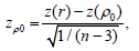 (4)
(4)
Where n is the sample size, z(r) is the Fisher z-transform applied to the sample value of the PCC, and z(ρ0) is the Fisher z-transform applied to the hypothesized value of the PCC. An approximate p-value is then obtained by calculating the appropriate tail probability for zρ0 using the standard normal distribution. For example, suppose one wishes to test Ho: ρ=0.2 vs. Ha: ρ ≠ 0.2, and that a sample of size n=30 yields r=0.52. Then
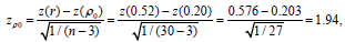
With an approximate two-tailed p-value of 2(1-Φ(1.94)) = 0.0522, where Φ(•) denotes the distribution function of the standard normal.
More generally, let ξ denote the population value of the measure of association to be tested (either the PCC, SCC, or KCC). Then a test statistic based on the Fisher z-transform is given by:
 (5)
(5)
| Measure of Association | b | c2 | Source |
|---|---|---|---|
| Pearson | 3 | 1 | [6] |
| Spearmana | 3 |  |
[2] |
| Spearmana | 3 | 1.06 | [7] |
| Kendall | 4 | 0.437 | [7] |
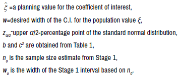
aFor sample size determination based on a confidence interval,  is a "planning value," where ρs denotes the population value of the Spearman rank correlation coefficient. For sample size determination based on a hypothesis test,
  is the null value ρs0. The value
 is used if
  ; otherwise 1.06 is used.
An approximate p-value is then obtained by calculating the appropriate tail probability for 0 zξ using the standard normal distribution.
Suppose we wish to use the test statistic in eqn. (5) to test
 (6)
(6)
Where -1 < ξ0< 1is the pre-specified null value of the desired measure of association (either the PCC, SCC, or KCC). Let ξ1 denote the alternative value of the measure of association that we wish to detect with our planned hypothesis test. For a two-tailed test of the null hypothesis in eqn. (6), the required sample size for detecting the value ξ1 with power φ using a test with significance level α is given by:
 (7)
(7)
Where zγ=upper γ-percentage point of the standard normal distribution,
z(•) denotes the Fisher z-transform, and
b and c2 are obtained from Table 1.
For a one-tailed test of eqn. (6), replace zα/2 in eqn. (7) by zα. If the formula in eqn. (7) does not yield an integer value, the next larger integer is used (Table 1).
A chart based on eqn. (7) for finding the sample size required to achieve 80% power for a two-tailed test of Spearman's coefficient at significance level 0.05 is given in Figure 1; charts for upper-tailed and lower-tailed tests of Spearman's coefficient are provided in Figures S1 and S2 in the Supplementary Materials. A chart for finding the sample size required to achieve 80% power for a two-tailed test of Kendall's coefficient at significance level 0.05 is given in Figure 2; a chart for a one-tailed test of Kendall's coefficient is provided in Figure S3 in the Supplementary Materials.

Figure 1a. Curves for finding the required sample size that will yield 80% power for a two-tailed test of a single Spearman coefficient at significance level 0.05, to be used when the alternative value (ρs1) is greater than the null value (ρs0). To use the chart, first locate the null value of the SCC along the x-axis. Then, draw a vertical line that intersects with the sample size curve corresponding to the desired alternative value. Finally, draw a horizontal line from the curve to the y-axis. The point of intersection with the y-axis is the required sample size.

Figure 1b. Curves for finding the required sample size that will yield 80% power for a two-tailed test of a single Spearman coefficient at significance level 0.05, to be used when the alternative value (ρs1) is less than the null value (ρs0). To use the chart, first locate the null value of the SCC along the x-axis. Then, draw a vertical line that intersects with the sample size curve corresponding to the desired alternative value. Finally, draw a horizontal line from the curve to the y-axis. The point of intersection with the y-axis is the required sample size.

Figure 2. Curves for finding the required sample size that will yield 80% power for a two-tailed test of a single Kendall coefficient at significance level 0.05. To use the chart, first locate the smaller of the null value (τ0) and the alternative value (τ1) of the KCC along the x-axis. Then, draw a vertical line that intersects with the sample size curve corresponding to the larger of τ0 and τ1. Finally, draw a horizontal line from the curve to the y-axis. The point of intersection with the y-axis is the required sample size.
Note that the sample size chart for the two-tailed test for the SCC (Figure 1) is formatted differently than that for the KCC (Figure 2). Because the value of c2 given in Table 1 for the SCC depends on the null value ρs0 if ρs0 < 0.95, the values of ξ1 and ξ0 do not enter the formula in eqn. (7) symmetrically, as they do for the KCC. Therefore, to simplify the sample size curves for the two-tailed test of the SCC, we split the chart into two pieces: one for alternative values of ρs greater than the null value ρs0 (Figure 1a) and one for alternative values of ρs less than the null value ρs0 (Figure 1b).
To use the sample size chart for the SCC, first locate the null value of the SCC along the x-axis in either Figure 1a (ρs0 < ρs1) or Figure 1b (ρs0 > ρs1). Then, draw a vertical line that intersects with the sample size curve corresponding to ρs1, the desired alternative value in the hypothesis test. Finally, draw a horizontal line from the curve to the y-axis. The point of intersection is the required sample size. To use the sample size chart for the KCC, first locate the smaller of the null value (τ0) and the alternative value (τ1) of the KCC along the x-axis. Then, draw a vertical line that intersects with the sample size curve corresponding to the larger of τ0 and τ1. Finally, draw a horizontal line from the curve to the y-axis. The point of intersection is the required sample size.
Suppose we are planning a study in which the SCC will be used as the measure of association and that we will test Ho: ρs=0.4 vs. Ha: ρs ≠ 0.4 once we have obtained the data. With a sample of n=129, we could detect an alternative value of ρs as small as 0.6 with 80% power using a two-tailed test with significance level 0.05 (Figure 1a). With a sample of n=180, we could detect an alternative value of ρs as large as 0.2 with 80% power using a two-tailed test with significance level 0.05 (Figures 1b and 2).
If we intend to use the KCC as the measure of association in the study being planned, the required sample sizes would be n=52 and n=75, respectively, for a two-tailed test of
assuming alternative values of τ1=0.6 and 0.2 (Figure 2). A comparison of the sample size results for the SCC and KCC in this example illustrates the phenomenon described by Helsel [5] that, with all other things (including sample size) being equal, smaller values of t, the sample value of the KCC, relative to r and rs are required to yield a given degree of statistical significance. With regard to sample size estimation in this article, this means that smaller sample sizes are required for the KCC than for the SCC to achieve the same level of power, all other things (including null and alternative values) being equal.
Sample size based on confidence interval estimation
The Fisher z-transform can also be used to derive approximate 100(1-α)% confidence limits for ρ. To obtain these limits, one must first derive a Wald-type approximate confidence interval (C.I.) for the Fisher-z transformed value of the population value of the PCC, z(ρ) = ln ((1+ ρ) / (1 - ρ)) / 2.
An approximate 100(1-α)% C.I. for z(ρ) is given by:
 (8)
(8)
where zα/2 is the upper α/2-percentage point of the standard normal distribution.
Next, the endpoints of the C.I. in eqn. (8) are "back transformed" using the inverse of the Fisher-z transform. This yields the following approximate 100(1-α)% C.I. for ρ:
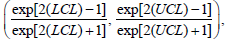 (9)
(9)
Where

More generally, let ξ denote the population value of the desired measure of association (either the PCC, SCC, or KCC). Then approximate 100(1-α) % confidence limits for z (ξ) are given by:
 (10)
(10)
Where b and c2 are obtained from Table 1. The limits in eqn. (10) are then back transformed using eqn. eqn. (9) to obtain approximate 100(1-α) % confidence limits for ξ.
Bonett and Wright [2] proposed a two-stage process for determining n based on the desired width of a two-sided 100(1-α)%
C.I. for the true value of a measure of association between two variables X and Y. This method can be applied to Pearson, Spearman, and Kendall coefficients.

if the desired confidence interval width has not been attained using n0. In these formulas,
If the value of n resulting from Stage 2 is not an integer, the next larger integer is used. Charts for finding the required sample size for estimating a SCC or KCC using a 95% two-sided C.I. that is based on this two-stage procedure are provided in Figures 3 and 4, respectively.

Figure 3. Sample size curves for finding the required sample size for estimating a Spearman coefficient using a 95% two-sided C.I. based on the two-stage procedure described in the text. To use the chart, first locate the planning value for the SCC along the x-axis. Then, draw a vertical line that intersects with the curve corresponding to the desired width of the confidence interval. Finally, draw a horizontal line from the curve to the y-axis. The point of intersection is the required sample size.

Figure 4. Sample size curves for finding the required sample size for estimating a Kendall coefficient using a 95% two-sided C.I. based on the two-stage procedure described in the text. To use the chart, first locate the planning value for the KCC along the x-axis. Then, draw a vertical line that intersects with the curve corresponding to the desired width of the confidence interval. Finally, draw a horizontal line from the curve to the y-axis. The point of intersection is the required sample size.
To use the charts in Figures 3 and 4, first locate the planning value for the measure of association along the x-axis. Then, draw a vertical line that intersects with the curve corresponding to the desired width of the confidence interval. Finally, draw a horizontal line from the curve to the y-axis. The point of intersection is the required sample size. For example, using the chart in Figure 3, we find that a sample size of n=177 would yield a 95% C.I. for ρs of width 0.20 based on a planning value of 0.70. For the KCC, a sample size of n=62 would yield a 95% C.I. for τ of width 0.20 based on a planning value of 0.70 (Figure 4).
Zero null value
By far the most commonly used null value in a test of a single PCC, SCC, or KCC, is ξ0=0. We have designed our charts so that it is relatively easy to determine the sample sizes required to detect several alternative values if the null hypothesis is H0: ξ0=0. For example, suppose that we are planning a study in which the primary analysis will be to perform a two-tailed test of H0: ρs=0. By simply reading the values from the y-axis in Figure 1a, we can identify the sample sizes needed for each of the alternative values given in Table 2.
| Alternative Value | 0.1 | 0.2 | 0.3 | 0.4 | 0.5 | 0.6 | 0.7 | 0.8 | 0.9 |
| Required Sample Size | 783 | 194 | 85 | 47 | 30 | 20 | 14 | 10 | 7 |
Negative coefficients
The sample size charts in this article can be used only when ξ1 and ξ0 have the same sign. For negative values of ξ1 and ξ0, one simply enters the appropriate chart with |ξ1| and |ξ0|. If ξ1 and ξ0 are of opposite signs, the formula in eqn. (7) is still valid; however, the charts provided in this article do not apply.
Minimum detectable alternative value
In addition to finding the sample size needed for planning statistical inference for Spearman or Kendall coefficients, the charts can also be used to find the minimum detectable alternative value for a given sample size. For example, suppose that the primary analysis in the study being planned will involve a two-tailed test of Ho: ρs=0.4 vs. Ha: ρs ≠ 0.4 at significance level 0.05, and that the largest possible sample size available to the investigators is n=50. One could determine the minimum detectable alternative value (ρs1) greater than the null value (ρs0 =0.4) from Figure 1a by first drawing a horizontal line from n=50 on the y-axis, and then drawing a vertical line from 0.4 on the x-axis. One then reads off the alternative values larger than 0.4 from this vertical line until it intersects with the horizontal line drawn from the y-axis. Note that graphical interpolation will be required if the horizontal line does not intersect with one of the sample size curves. Using Figure 1a, we see that with n=50, we could detect any alternative value ρs1 greater than or equal to 0.7 with 80% power using a two- tailed test with significance level 0.05. A similar method could be used with Figure 1b to determine the maximum detectable alternative value (ρs1) less than the null value in a test of Ho: ρs=ρs0 vs. Ha: ρs ≠ ρs0.
Interpolation errors
As with any graphical method, these charts are subject to error. For example, one must interpolate graphically if the horizontal line drawn from the appropriate curve in the charts intersects the y-axis at a value between tick marks. This is more of a problem for larger sample sizes since the distances between tick marks are much larger. However, the error for the interpolated value will be no larger than the difference between the values corresponding to the tick marks, and an adjustment can be made by slightly inflating the value read from the charts. We have found that an 6-inch ruler marked off in millimeters is particularly useful for carrying out any necessary graphical interpolation in the charts.
In this article, we have presented charts that can be used for sample size determination when planning a study in which the primary analysis involves hypothesis testing or confidence interval estimation for a Spearman or Kendall coefficient. In addition to the charts, we have provided simple sample size formulas that can be used for more accurate calculations. We have found Microsoft Excel© to be particularly useful for performing these calculations, and a spreadsheet that accomplishes this is available from the second author. Freely available SAS code for performing these sample size calculations can be found in the on-line Software Appendix for Looney and Hagan [8], which can be downloaded from http://bcs.wiley.com/he-bcs/Boo ks?action=index&itemId=1118027558&bcsId=9351.
Despite the widespread use of correlation analysis, it is generally the case that little or no attention is given to sample size determination when planning a study in which correlation will be the primary analysis.
In fact, our review of clinical research journals indicated that none of the 111 articles published in 2014 that used correlation as the primary analysis provided a sample size justification or power calculation. It is hoped that availability of the tools presented in this article will encourage analysts to perform sample size calculations for correlation coefficient inference. It is vitally important that one do this, given the adverse consequences when studies are either under- or over-powered. This can easily happen if one does not perform a sample size calculation prior to beginning the study.
Journal of Biometrics & Biostatistics received 3496 citations as per Google Scholar report