The Impact of Remittances on the Living Conditions of Households (Evidence from Kebri Dehar City, Ethiopia): Propensity Score Matching Model (PSM)

Walelign Amenu Zeleke^*
*Correspondence: Walelign Amenu Zeleke, Department of Global Economics, Indian Institute of Management Calcutta, West Bengal, India, Email:

Keywords

Counterfactual • Kebri dehar • Living condition • Propensity score matching Model • Remittance

Introduction

Migrants who migrate overseas or to urban areas in their nation frequently send money to families in their home countries and this money is used to help them meet basic needs and secure their livelihoods [1]. Remittances impacted positively on the living conditions of recipient households’ by improving lifestyle, solemnizing marriages in well-established families, schooling children at reputed institutions, constructing cemented houses, purchasing landholdings and new brand vehicles, generating divergent income activities at a household level, and investing in real estate etc. [2]. Remittance flow that smooth consumption and enables households to invest in human and other resources could significantly improve the living conditions of receiving households [3]. Remittance flows to Low and Middle Income Countries (LMICs) are estimated to be a total of UD$ 442 billion in 2016, an increase of 0.8 percent over the past year. LMICs are mostly from Asia, Latin America, Eastern Europe, and Africa [4]. This source of household income might have a substantial impact to improve the living conditions of people in poorer parts of the world [5]. Ethiopia has experienced interrelated socio-economic and political crises that have led to a massive exodus of people, both internally and across borders. In terms of foreign exchange generation capability, remittances constitute an important source of foreign currency for Ethiopia, perhaps even more than export revenues [6]. According to recent World Bank data, the largest destinations for Ethiopian migrants among high-income countries in 2010 were the United States, Israel, Saudi Arabia, Canada, and Germany [7]. According to the World Bank, Ethiopia is the eighth-largest recipient of remittances in Sub-Saharan Africa, with inflows increasing considerably in recent years, from 46 million USD in 2003 to an estimated 387 million USD in 2010 [8]. Ethiopian-Somali diaspora organizations have reached an agreement with their relatives back home on financial matters [9]. The remittances members of the Somali diaspora send to their poor family members each year to provide food, shelter, clothing, schooling, health care, and other necessities [10]. The general manager of Dahabshiil Jigjiga office, a major Somali money transfer, and banking institution said that at least 100 to 150 people visit the branch every day to collect money transfers sent by diaspora senders. Typically, each of these receives between $100 and $150 USD. Other branches in towns such as Kebridehar, Deghabur, Gode, and Ras may be similarly pretentious[11]. Given this Kebri Dehar has one of the highest remittance inflows in Somali regional state ; the goal of this study is to investigate if remittance has a significant impact on the living conditions of households in Kebri Dehar by taking into account main household level determinate variables.

Statement of the problem

One of the most argumentative issue in today's academic world is the relationship between worker remittances and economic growth, with some arguing in favor and others arguing against it [12]. Transfers of funds from emigrants to their home societies, known as migradollars, might have long-term positive impacts on recipient nations if the funds are invested in productive projects [13]. Despite potential for growing economic inequalities, empirical studies show that remittances can help reduce poverty and improve household and community living conditions [14]. According to Andersson the findings to investigate the effects of foreign remittances on the living condition of households in rural Ethiopia had a significant positive influence on household subjective well-being [15]. The impact of overseas remittances on economic growth in Ethiopia was investigated using the Autoregressive Distributed Lag Approach (ARDL). The findings of the studies demonstrated that foreign remittance had a favorable and considerable long-run growth impact. However, the short-run impact was found to be negative and statistically significant [16]. Households in Ghana, on the other hand, regard remittances as any other source of income, and remittance income has little effect on their marginal expenditure [17]. This study analyzes the impact of remittances on the living condition of households in Kebri Dehar city. It uses the Propensity Score Matching Model (PSM estimation technique) to analyze cross-sectional data.

Review of related literature

Remittances enable better education, healthcare and other determinants of living conditions, say experts [18]. Remittances from overseas are critical to the survival of communities in many developing nations, according to a study by the World Bank and IMF published in 2007 [19].

Empirical literature review

The impact of remittances on economic outcomes including growth, inequality, income distribution, poverty, and population health has been extensively studied [20]. A recent study on Turkish remittances concluded that consumption smoothing is an important short-run motive for sending remittances to Turkey [21]. In Hargeisa, Somalia, Lindley equally found that migrants tend to send more remittances from abroad when the family experiences a decline in fortunes [22]. They also have a positive impact on household welfare, food, health, and living conditions in their host countries, according to studies [23]. Evidence suggests that remittances from abroad are crucial to the survival of communities in many developing countries as indicated in an IMF country analyses report by [24]. In this report, it was found that once survival needs are satisfied; migrants do use remittances for investment purposes including education, housing, and small scale enterprise [25]. In Ghana, remittances improve household living condition and minimize the effects of economic shocks to household wellbeing, although it is not able to offset the shocks completely except for food crop farmers (the poorest in Ghana) [26]. Microeconomic research has revealed that socioeconomic variables of migrants and recipient households, such as income, education, and risk exposure, influence the likelihood of sending and receiving remittances. According to Lucas and stark; Vanwey, under the assumption of altruism, these studies show that the likelihood of sending remittances and the amounts transferred are increasing functions of migrant income [27].

Conceptual framework

Specific correlations between remittances and household living conditions can be drawn based on the theoretical and empirical literature examined thus far (Figure 1).

Materials and Methods

Research design

According to Boru using a mixed research approach or when both quantitative and qualitative data gathering techniques and analytic procedures are employed in study design. This study should be conducted using a mixed method to examine the impact of remittances on the living conditions of households in Kebri Dehar city.

Data type and source

Both primary and secondary sources of data would be used to obtain the necessary information for the impact of remittance on the living condition of households in Kebri Dehar.

Secondary data had been gathered from a variety of sources, including prior studies, articles, thesis and research papers, firm records or archives, government publications, industry analysis by the media, websites, the Internet, and other sources.

Sample size and sampling techniques

Any study or investigation whose purpose is to draw conclusions about the population from a sample must take the sample size into account [28]. Cochran's formula is particularly useful in cases where the population is unknown and large [29].

The Cochran formula is:

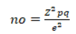
Where,

no=Sample size,

Z=Selected critical value of desired confidence level,

p=Estimated proportion of an attribute that is present in the population,

q=1-p and e=Desired level of precision (i.e. the margin of error).

Since the researcher was doing a study on the impact of remittances on the living conditions of households in Kebri Dehar city. So p=0.5 the researcher want 95% confidence, and at least 5 percent-plus or minus-precision. A 95 % confidence level gives us Z values of 1.96, (the z-value is found in Z table) per the normal distribution tables, so we got it:

The study was conducted in Kebri Dehar city due to the high remittance receiving area and then a two-stage sampling technique was employed for respondents. The total sample sizes of 384 households were drawn based on whether the household received remittances or not, time of establishment and household living conditions. To address the study's specific objective, randomly selected households from both categories, Non-Remittance Receiving Households (NRRHs) and Remittance Receiving Households (RRHs), were asked. It is collected from residential areas, private colleges, banks, and other public places such as recreation centers and internet cafes, where migrant families are supposed to spend their time and use services. However, out of the total of 384 households, only 340 of the sampled households appropriately respond to the given questions. The rest of 44 households have reduced the questioner either because they reject to respond to the questionnaire or don’t bring a tangible answer.

Instruments of data collection

Questionnaires, interviews, and observation would have been used as research instruments or data tools in this study.

Model specification

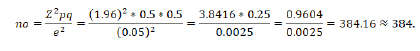
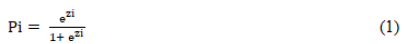
The researcher used propensity to solve potential bias due to unobserved parameters and the model is estimated in two stages: In the first stage, estimating Logit or Probit models whether households receive remittances as binary dependent variables. In the second stage, look at the effect of treatment on the outcome of matching remittances received by non-receiving households. The propensity score is the conditional probability of receiving a treatment given pretreatment characteristics. Ri(i=1 and 0) is the binary variable equal to 1 household receiving remittances and otherwise 0. As described by Rosenbaum and Rubin, matching can be performed conditioning on P(X) alone rather than on X, where P(X) ≡ Pr(D=1|X=E(D|X) is the probability of participating in the program conditional on X. The treatment variable in the Logit or probit model is remittance, which has a mathematical value of 1 if a household receives a remittance and 0 otherwise.

Where, P_i is the probability of i^th households who receives remittance and it ranges from 0 to 1.

Where,

β₀=Intercept, i=1, 2………n,.

β_i=Regression coefficients to be estimated or Logit or probit parameter,

X_i=Pre-intervention characteristics and R=1 means the household receiving remittance,

Ui=A disturbance term.

There is a problem with non-linearity in the previous expression, but this was solved by creating the odds ratio then the probability that the household belongs to non-remittances receiving group is given by:

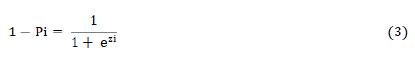
Then the odd ratio can be written as:

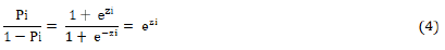
The left side of equation (4), (Pi/(1-Pi)), is simply the odds ratio in favor of receiving remittance. It is the ratio of the probability that the household would receive remittance to the probability that it wouldn’t receive remittance. By taking the natural log of equation (4), the log of odds ratio can be written as:

Where,

Li- is the log of the odds ratio in favor of participation in remittance which is linear both in Xi and parameters.

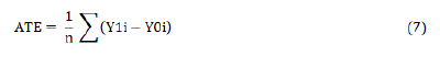
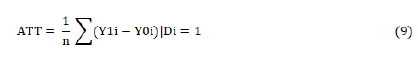
The odds ratio could be interpreted as the probability of something happening to the probability it won’t happen. Once the propensity score is computed and the model used by Zaid is followed, the impact of treatment on outcome say (Y) can be stated as: Let’s say we have an individual receiving remittance and some others who are not, and denoting the outcome variable of the treated individual by (Y1i) and that of the non-treated by (Y0i), it should put the effect of treatment as (Y1i-Y0i). For a group of individuals, one has to use the mean of outcomes across all the receiving remittance and nonreceiving remittance, which has been then give us the expected value or average effect of treatment. In the evaluation literature, this is known as Average Treatment Effect (ATE), according to Fitsum Aklilu, cited by Wooldridge, Cameron and Trivedi (Fitsum). Thus, for a population we have the following with “E” standing for expected value or mean:

The sample equivalent of the above equation is given as follows:

Where,

ATE represents the average difference in outcomes between households with remittances and households without remittances.

Y1i=Outcome of an individual treated by the program (remittancereceiving households)

Y0i=Outcome of non-treated (non- remittance receiving households)

D=Dummy variable, where D=1 shows remittance-receiving households and D=0 shows non- remittance receiving households and n=Number of observations

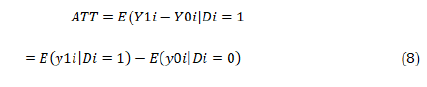
As a result, the researcher employs ATT to evaluate the impact of remittances on household living conditions. Accordingly, the impact is calculated as the difference between what is happening to remittance recipients and what would have happened if they had not received remittance.

Where,

Di, is the remittance dummy taking the value of 1 if the household receiving remittance and 0 if other way. Thus E (Y1i|Di=1) represents the expected outcome of remittance receiving households and E (Y0i| Di=0) represents the unobserved outcome of remittance receiving households had they not received remittances. The counterfactual estimates represent what the outcome of remittance receiving households would emittance receiving activities.

E-indicates the expected (average) value. The sample equivalent is given as:

The factual outcome with remittance (Y1i|Di=1) is observable for household receiving remittance but here the problem is the counterfactual outcome for household without receiving remittance (Y0i|Di=0) is not observable for the same household as it is impossible to get the same individual with and without receiving remittance simultaneously. The propensity score is the probability of receiving remittances (X), conditional on a set of characteristics, (X) such that P(x)=Pr(D=1|X)=E(D|X). In general, impact estimates could be enhanced if data is available before and after treatment, allowing the outcome to be stated in terms of a change in outcome before and after treatment. If E (Y1i|D=1) and E(Y0i|D=0) were equal, there couldn’t be any variation between what we want to measure and what we observe making our impact evaluation a straight forward task.

Conditional Independence Assumption (CIA)

Conditional independence states that given a set of observable covariates X that are not affected by treatment; potential outcomes Y are independent of treatment assignment T. Conditional mean independence requires that, given (X), the mean outcomes for households in the control group are identical to mean outcomes for treated households had they not been treated.

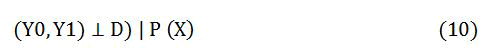
Equation (10) says outcome and participation are independent given the propensity score P(X). Common support region assumption and balancing condition

The common support is the region where the balancing score has positive density for both treatment and comparison units. That is: 0

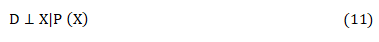
Where P(X) the propensity score computed on the covariates equation (11) is explained as; the PSM estimator is the mean difference in outcomes over the common support, appropriately weighted by the propensity score distribution of the receiver.

If equation (11) is fulfilled, observation with a similar propensity score will have an identical distribution of observable and unobservable characteristics irrespective of treatment. Once the propensity score is calculated and the balancing condition is met, impact or ATT can be estimated as shown in equation (12) below. Using the propensity score to deal with selection bias, equation (8) is thus modified as:

Several matching techniques have been developed to match households based on the estimated propensity score.

In Nearest Neighbor matching (NN): a controlled household is matched with a treated household based on the closest propensity score. The number of matching partners in NN matching can be varied such that a treated household is matched with the n closest neighbors.

Kernel matching: Another option is the kernel matching estimator that matches the treated households with a weighted average of all controls, using weights that are inversely proportional to the distance between the propensity scores of the two groups.

Caliper/radius matching: The above discussion tells that NN matching faces the risk of bad matches if the closest neighbor is far away. To overcome this problem researchers use the second alternative matching algorism called caliper matching.

Stratification or interval matching: This procedure partitions the common support into different strata (or intervals) and calculates the program’s impact within each interval.

Results and Discussion

Descriptive analysis

Socio-economic and demographic characteristics: The households are classified into two groups namely remittances receivers and non-remittances receivers. Qualitative characteristics (dummy variables) are expressed in terms of frequency or percentage while the continuous variables are compared in terms of mean and standard deviation.

As shown in Table 1, females are more signified than males, although females are more represented in Remittance Receiving Households (RRHs) than in Non-Remittance Receiving Households (NRRHs). Married couples make up 75.355% of the total asked households in all categories. The majority of them are Muslims, followed by orthodox and protestants. Catholics are the religious group with the lowest representation in NRRHs. In terms of asset ownership, houses were owned by 64.035% of all households, 59.50% of RRHs, and 68.57% of NRRHs. In terms of employment categories, self-employment is higher in RRHs than NRRHs and unemployment are higher in NRRHs compared to RRHs although the reverse is true for the category of homemakers and pensioners. RRHs are to some extent older than NRRHs and also, the dependency ratio is higher in RRHs than NRRHs. The mean level of education shows that most of the respondents are educated although NRRHs are extremely educated than their RRHs counterparts. Mean family size is larger in remittance recipients than non-recipients. Looking at the log of the outcome variables there is a difference in the mean income and expenditure among the two groups. All outcome variables (household income, consumption expenditure, and food expenditure) are higher in RRHs compared to NRRHs.

Table 1. Socio-economic and demographic characteristics of households or (dummy variables).

Econometrics result

Estimation of propensity scores: The treatment variable was remittances it was a dummy that shows remittances receiving households and non-remittance receiving households. Results presented in Tables 2 and Table 3 shows the estimated model appears to perform well for the intended matching exercise. The pseudo-R^2 value is 0.0142. According to Pradhan and Rawlings, a low R^2 value shows that the allocation of the program has been defacto random. In other words, a low R^2 value means that remittance receiving households do not have many distinct characteristics overall and as such finding a good match between remittance receiving and non- remittance receiving households becomes easier. The pseudo-R^2 indicates how well the regressors explain the participation probability.

Table 2. Algorithm to estimate the propensity score.

Estimation of the propensity score

Iteration 0: log likelihood=-230.3481

Iteration 1: log likelihood=-227.07651

Iteration 2: log likelihood=-227.07584

Probit regression

Number of obs=340

LR chi square (9)=6.54

Prob>chi square=0.6844

Log likelihood=-227.07584

Pseudo R²=0.0142

Table 3. Probit regression results.

Estimation of the propensity score Iteration 0: log likelihood=-230.3481 Iteration 1: log likelihood=-227.07651 Iteration 2: log likelihood=-227.07584

Probit regression Number of obs=340 LR chi square (9)=6.54 Prob>chi square=0.6844 Log likelihood=-227.07584 Pseudo R2=0.0142

As shown the above Table 3, the impact of remittances on the living conditions of households was significantly influenced by nine explanatory variables. The probit estimation results, when looked into the estimated coefficients (Table 3), indicate that program participation is significantly influenced by five explanatory variables. Gender, employment status, age, automobile truck, and household sizes are significant variables that affect remittance receiving households to the program. The common support region would then lie between (.39069254, .73591771). In other words, households whose estimated propensity scores are less than 0.39069254 and greater than 0.73591771 are not considered for the matching exercise. As a result of this restriction, there have not been any nonremittances receiver and remittances receiver households were discarded from the analysis.

Gender of household: As we have seen in the result above, it has a negative impact and is statistically significant on the probability of receiving remittances because households with a female head were more likely to receive remittances compared to their male headed counterparts. This result could be misleading unless we take care of the fact that most of these female headed households had male migrant heads that used to be the household heads, and in the absence of them, their wives acted as household heads.

Employment status: It has a positive impact and is statistically significant due to households with relatively large numbers of employed members being expected to generate more income to smooth consumption and if they are unemployed they migrate and they send remittance funds towards their families and these remittance funds reduce unemployment in their families.

Age of household: It has a positive impact and is statistically significant on the likelihood of receiving a remittance since remittance-receiving families have more children and older people than the control group, whereas households without remittances have a lower likelihood of having younger people in their households than those who do. According to Hamel, as quoted in Borici and Gavoci, older people receive more remittances compared to younger people.

Households’ owners of house: Physical asset ownership, such as houses, automobiles, or trucks, has a negative impact on the likelihood of getting remittances since owners are better off and less reliant on remittances in bad times.

Dependency ratio: Measures the ratio of family members aged below 15 and above 64 to the rest of family members. Households with a large number of dependents are poor and resort to transfers during times of shocks.

Level education: It has a negative and highly insignificant result for our main variable of interest in the probability of receiving remittance.

Household head education level is expected to affect remittance negatively because the more educated are expected to generate more income that could reduce remittance dependency.

Bank visit: It has a positive impact on the probability of receiving remittance because households receive remittance frequently they visit a bank.

Household family size: It has a positive and significant impact on the probability of receiving remittance. As the household size increases the likelihood of receiving remittance would also increase because members of the household migrate abroad and tray to help their families who live in their origin (Table 4).

Iteration 0: EE criterion=4.583e-21
Iteration 1: EE criterion=5.288e-23
Treatment-effects estimation
Number of obs=340
Estimator: Augmented IPW
Outcome model: Linear by ML
Treatment model: Probit

Table 4. Treatment-effects estimation/ATE.

On average remittance receiving households if all households were to receive would be 1657.402 birrs greater than the average of 58806.53 birrs that would occur if none of the households had received (Table 5).

Table 5. On average remittance-receiving households.

On average remittance-receiving households if all households were to receive would be 4037.812 birrs for food expenditure greater than the average of 42720.06 birrs for food expenditure that would occur if none of the households had received (Table 6).

Table 6. If all households were to receive would be 3229.107 birrs.

The POM for treatment level t is the average potential outcome for that treatment level:

POMt=E (yt)

On average remittance receiving households if all households were to receive would be 3229.107 birrs for consumption expenditure greater than the average of 41732.56 birrs for consumption expenditure that would occur if none of the households had received.

A treatment effect is a change in the outcome caused by an individual getting a treatment (remittance) instead of another. We cannot estimate individual level treatment effects but average treatment, because we observe only each getting one or another treatment. Average Treatment Effect (ATE) measures the effect of remittance on the whole sample of households. When the distribution of a covariate does not vary over the treatment levels, the covariate is said to be balanced. The distribution of the household concerning estimated propensity scores is depicted in Figure 2 below it shows that the majority of treatment households are found on the right side of the distribution, partly in the middle, and partly on the left. On the other hand, most control households are spread across the distribution, with some in the center and some on the left.

Balance of propensity score and covariates testing: As known before, the purpose of the propensity score estimation is not only to obtain a specific forecast of selection into treatment but also to balance the distributions of relevant variables in both groups. The mean standardized bias for matching and unpaired samples is shown in Table 6 (5^th column). The matching technique displays the total bias reduction in column six. In the present matching models, the standardized difference of covariate before matching is in the range of 1.3% to 21.4 % in absolute value. The remaining covariate standardized difference after matching lies between the range of 0.1% and 19.0%. The standardized difference of covariates of the unmatched is significantly greater than the standardized bias of the matched. Matching creates the readiness of covariates for use in estimation through balancing treatment and untreated samples. Before the study took a match between the covariates, t stats showed almost half of the covariates displayed differently statically significant. On the other hand, after matching, all covariates were balanced(Table 7).

Table 7. Propensity score and covariate balance.

Table 8 confirms that Pseudo-R² and LR chi square among matched and unmatched households, the matched household Pseudo-R²=0.015 is low and LR chi square=7.75 are insignificant likelihood ratios tests. This supports the theory that both groups (remittance receiver and non-remittance receiver) have the same distribution of covariates X after matching. The treated and control groups are balanced through a matching procedure. Similar observed characteristics make it easy to assess the impacts of remittances on the living conditions among control and treated groups with their common support.

Table 8. Chi square test for the joint significance of variable.

Estimating treatment effect on treated: To generate a robust ATT, the researcher used four different types of matching criteria. First, the researcher applied a nearest neighbor matching criterion, which matches remittance receiving households with non-remittance receiving households with the closest propensity score. The counterfactual match for each remittance receiving household was then constructed using a kernel matching criterion, which uses a weighted average for non-remittance receiving households [31-33]. If the closest neighbor is far away and to overcome this problem researchers use the caliper matching and then caliper matching is an individual from the comparison group is chosen as a matching partner for a treated individual that lies within a given caliper (propensity score range) and is closest in terms of the propensity score. Finally, to match treated and control observations, the researcher used a stratification criterion. This form of matching criterion divides observations into strata and then matches observations that are comparable within each stratum (stratified matching criterion). It's worth noting that in propensity score matching, the variance for the treatment effect is estimated incorrectly [34]. Nevertheless, correcting this problem is straightforward by bootstrapping the standard errors [35]. Therefore, bootstrapped standard errors with 5 replications are estimated for the treatment effect for two matching criteria, kernel, and stratification. The result suggests that for every matching algorithm, the ATT is positive and significant, which means that remittances account for a positive and statistically significant difference between the matched treated (remittance-receiving) and control groups in terms of per capita income, consumption expenditure, and food expenditure in all matching algorism. The results in a Table 9 shows that the receiving of remittances is positively and significantly affects households’ income per capita in the study area. This shows that the household income per capita for remittance receiver households on average; 8821.255 birrs in the case of Nearest Neighbor (NN) matching, 6637.047 birrs in the case of caliper/radius matching, 4782.573 birrs in kernel matching, and 2740.511 birrs in the case of stratification/ interval matching. So we can be generalized that remittance receivers were found high income per capita than non-receivers in the study areas. Given the average household income per capita (57298.675) the increment is significant at 1% for all four matching algorisms. The results from the four matching algorithms confirm that receiving of remittance higher income per capita on average with ranges of 8821.255 birr in the case of Nearest Neighbor (NN) matching to 2740.511 birr in the case of stratification/interval matching algorithm. In other words, the remittance receiver households were found better by getting higher income due to remittance (it considers as extra income sources) than non-receiver households in the study area. This finding has been supported by Muhammad Azam and Syed Ali Raza; he found that remittance has a positive impact on the household’s income per capita in Pakistan and he concludes incomes of remittance receiver households in Pakistan are higher than a non-remittances receiver household.

Table 9. Result of boot strap propensity score matching.

Conclusion

The impact of remittances on the living conditions of recipient households in Kebri Dehar city has been analyzed using crosssectional data. The primary data were collected from 384 households from both remittance receiver and non-remittances receiver households using a structured questionnaire by using a two-stage sampling technique. The total of 384 households, only 340 of the sampled households appropriately respond to the given questions. The rest 44 households have reduced the analysis either because they reject to respond to the questionnaire or don’t bring the tangible answer. As a result, from 340 sampled households 200 households were receiving remittances and the remaining 140 are Non- Remittances Receiving Households (NRRHs).

A propensity score matching technique, which has become the most extensively used non-experimental tool for social program impact evaluation. In the absence of baseline data, it is used to extract comparable pairs of treatment-comparison households in a non-random program structure. Furthermore, it could account for but not eliminate selection bias and estimate counterfactual effects.

A descriptive statistic was applied before running regression analysis to establish some useful comparisons between remittance receiving and non-remittance receiving households. The descriptive analysis displays significant differences between the recipient and non-recipient households concerning the mean value of the log of total consumption expenditure; log of food expenditure and log of per capita income. The mean values of the three outcome variables household income, consumption, and food expenditure are higher in remittance-receiving households compared to non-remittance receiving households.

There is also the basic difference in Socioeconomic and demographic characteristics of households. For example, remittance recipients are older but less educated than non-remittance recipient households. This implies that the older-aged population is more dependent while the educated households mostly have stable incomes and require less support of remittances.

Approximately 86 percent of these remittances are sent in the form of cash. Remitted monies are mainly obtained from sisters and brothers through blood ties and strategic agreements between a migrant and his family. The implication is that migration is a strategic decision to send a migrant abroad to improve the household living condition.

All independent variables have the expected signs, except gender and automobile truck both are significant but negative. Household size and age have positively correlated with receiving remittances and are statistically significant. A higher education level decreases the probability of receiving remittances and compared to no formal education which is the baseline here all levels of education, from incomplete primary up to secondary or higher education decrease the probability that the household receives remittances.

The living condition benefits for both remittance-receiving households and non-remittance receiving households had they received are estimated using a treatment effect model. Significant and positive values of ATT were found on the three outcome measures (income, consumption, and food expenditure).

Recommendations

Remittances in Kebri Dehar city have a positive impact on the living conditions of households. Investment at the national level by such families was invisible due to a lack of guidance either by the government or other sources. This study recommends that the government and other concerned bodies need to mobilize the heads of the recipient families to utilize remittances in the national interests. Empirical results show that appropriate policy to explore more foreign employment and more proficient use of remittances would help the living conditions of households. In this regard, some policy considerations under different objective headings are offered below.

• The financial sector should be developed and the channels of remittances should be diverted and controlled the informal sector to reduce costs and better benefit from remittances.

• The government should be collaborating with banks and money transfer agents should devise appropriate policies and strategies in order to diversify payment instruments, for instance, every bank made payments to their customers only in birr notes, no way to get dollars except black market.

• Since it is good to work abroad to bring better living conditions to one family since the government should improve and strengthen its relationships with the rest of the world, especially major origins of remittances.

• Although remittance is good to improve the living conditions of households, the government and other stakeholders should bring opportunities to invest the remitted money in order to reduce remittance dependency.

• We recommend that better quality of institutions and city.

• Administrations required which improve the living condition of households result in effective utilization of remittance and maximize household’s well-being.

• Promoting infrastructure, reducing uncertainty, and creating a favorable environment for more productive use of remittances to establish well-improved living conditions for households.

References

1. Adams RH. "International Remittances and the Household: Analysis and Review of Global Evidence." Working paper WPS 4116, (2006.)
2. Adams JR and Richard H. "Remittances, Consumption and Investment in Ghana." World Bank Policy Research Working Paper No. 4515, (2008). [Google Scholar]
3. Ahmed B and Haji J. "Impact of Small-Scale Irrigation on Farm Householdsâ?? Technical Efficiency: The case of Eastern Oromia, Ethiopia." Asian J Agric Biol 2 (2014): 224â??234. [Google Scholar]
4. Ajefu JB. "The Effects of International Remittances on Expenditure Patterns of the Left-Behind Households in Sub-Saharan Africa." Rev Dev Econ 2019 (2021): 405â??429. [Crossref] [Google Scholar]
5. Alper AM and Neyapti, B. "Determinants of Workerâ??s Remittances: Turkish Evidence from High-Frequency Data." East Eur Econ 44 (2006): 91â??100. [Crossref] [Google Scholar]
6. Andersson L. "Migration, Remittances and Household Welfare in Ethiopia." Working Paper Series, 31. 2014-004, United Nations University-Maastricht Economic and Social Research Institute on Innovation and Technology (MERIT), (2012). [Google Scholar]
7. Becker SO and Ichino A. "Estimation of Average Treatment Effects Based on Propensity Scores." 4 (2002): 358â??377. [Crossref] [Google Scholar]
8. Berhanu K. "The Politica Economy of Diaspora Remittances in the Ethipian Somali Region." DIIS Working Paper No. 2019:9, (2019).  [Google Scholar]
9. de Haas H. "Remittances, Migration and Social Development." Social Policy and Development Programme Paper Number 34, 34, 46. (2007). [Google Scholar]
10. Dilip R. "Workersâ?? Remittances: An Important And Stable Source of External Development Finance." Global Devel Finan (2003): 19. [Google Scholar]
11. Fitsum A. "Assessing the Impact of Productive Safety Net Program on Asset Building and Sustainable Land Management Practices: A Cross-Sectional Analysis from Eastern Hararghe, Haramaya. de Boeck Brussels." Mekelle University, Ethiopia, (2013). [Google Scholar]
12. Getachew B. "Remittances and Household Welfare: Longitudinal Evidence from Urban Ethiopia." School of Graduate Studies Department of Economics Remittances and Household, (2008).
13. Giorgis KG and Molla M. "The Impact of International Remittance on Poverty, Household Consumption and Investment in Urban Ethiopia: Evidence from Cross-Sectional Measures." Ethiop J Econ 22 (2013): 63-108. [Google Scholar]
14. Goldring L. "Family and Collective Remittances to Mexico: A Multi-Dimensional Typology." Dev Change 35 (2004): 799â??840. [Crossref] [Google Scholar]
15. Hameli K. "The Impact of Remittance on Households: The Case with Residents of Prizren Region."  Prizren Soc Sci J 2 (2018): 1â??11. [Google Scholar]
16. Kifle MT. "The Role of International Remittance on Economic Growth in Ethiopia: An Autoregressive Distributed Lag Approach." Addis Ababa University, Ethiopia, (2014).
17. Kollner and Sebastian. "Remittances and Educational Attainment: Evidence from Tajikistan." Discussion Paper Series 124, Julius Maximilian University of Würzburg, Chair of Economic Order and Social Policy, (2013). [Google Scholar]
18. Kr Sarmah H, Sarmah HK, Bora Hazarika B and Choudhury G, et al. "An Investigation on Effect of Bias on Determination of Sample Size on the Basis of Data Related To the Students of Schools of Guwahati." Int J Appl Math Stat scien 2 (2013): 33â??48.
19. Kuschminder K, Andersson L and Seigel M. "Migration and Multidimensional Well-Being in Ethiopia: Investigating the Role of Migrants Destinations." Migr Dev 2324 (2018): 1â??20. [Crossref] [Google Scholar]
20. Lopez-Videla B and Machuca CE. "The Effects of Remittances on Poverty at the Household Level in Bolivia: A Propensity Score Matching Approach. Polit." Publicas 2 (2014): 7â??22. [Google Scholar]
21. Muhammad N, Ahmad M, Ahmad N and Shah M, et al. "Socio-Economic Conditions of Households (a Case Study of Rural Areas in Dir Lower, Nwfp)." Sarhad J Agric 26 (2010): 141â??145.
22. Maimbo SM and Ratha D. "Development Impact and Future Prospects (Issue c)." World Bank Publications, Pennsylvania Ave. NW, Washington, D.C. (2005): 378. [Google Scholar]
23. Neilson T. "King of charcoal: Japanese Create New Life for Dying Industry." In Inwood Magazine 2 (2011): 32â??33.
24. Nilsen J. "Remittances and Developmentâ?¯: The Impact of Remittances on Livelihood Security." Evidence from Ko Kaeo Sub- -district, Thailand. Thailand, (2014). [Google Scholar]
25. Ozden C, Parsons CR, Schiff M and Walmsley TL, et al. "Where on Earth is Everybody? " The Evolution of Global Bilateral Migration 1960-2000. World Bank Econ Rev 25 (2011): 12â??56. [Crossref]
26. Politis DN. "The Impact of Bootstrap Methods on Time Series Analysis." Stat Sci 18 (2003): 219â??230. [Crossref] [Google Scholar]
27. Quartey P and Blankson T. "Do Migrant Remittances Minimize the Impact of Macro-volatility on the Poor in Ghanaâ?¯?" Middle East 1991(2004a): 1â??32.
28. Quartey P and Blankson T. "Do Migrant Remittances Minimize the Impact of Macro-volatility on the Poor in Ghanaâ?¯?" By Final Report Submitted to the Global Development Network (GDN). Middle East 1991 (2004b): 1â??32.
29. Quartey P and Quartey P. "The Impact of Migrant Remittances on Household Welfare in Ghana." AERC Research Paper 158, African Economic Research Consortium, Nairobi, (2006): 1-37. [Google Scholar]
30. Muhammad A and Raza SA. "Do Workersâ?? Remittances Boost Human Capital Developmentâ?¯?" Pak Dev Rev 55 (2016): 123â??149. [Google Scholar]
31. Sunny J, Parida JK and Azurudeen M. "Remittances, Investment and New Emigration Trends in Kerala." Rev Dev Chan 25 (2020): 5â??29. [Crossref] [Google Scholar]
32. Tambo J and Wünscher T. "Beyond Adoption: Welfare Effects of Farmer Innovation Behavior In Ghana." ZEF-Discussion Papers on Development Policy, (2016): 216. [Google Scholar]
33. Wadood SN and Hossain A. "Microeconomic Impact of Remittances on Household Welfare: Evidences from Bangladesh." Bus Econ Horiz 13 (2017): 10â??29. [Crossref] [Google Scholar]
34. Wolde TG. "Impact of Remittance on Rural Household â?? s Welfareâ?¯: Evidence from North Wollo Zone, Gubalafto Woreda in Amhara Regional State, Using IV- Estimation Technique." Glob Econ J 6 (2018): 1â??6. [Crossref]
35. Kinati W, Bekele A and Chinnan KPM. "Impact of Farmer Research Group Interventions on Maize Farmers in Central Rift Valley of Oromia: An empirical study." J Agric Ext Rural Dev 6 (2014):  94â??107. [Crossref] [Google Scholar]